当前位置:网站首页>Common optimization methods
Common optimization methods
2022-07-05 05:33:00 【Li Junfeng】
Preface
In the training of neural networks , Its essence is to find the appropriate parameters , bring loss function Minimum . However, this minimum value is too difficult to find , Because there are too many parameters . To solve this problem , At present, there are several common optimization methods .
Random gradient descent method
This is the most classic algorithm , It is also a common method . Compared with random search , This method is already excellent , But there are still some deficiencies .
shortcoming
- The value of step size has a great influence on the result : Too many steps will not converge , The step size is too small , Training time is too long , It can't even converge .
- The gradient of some functions does not point to their minimum , For example, the function is z = x 2 100 + y 2 z=\frac{x^2}{100}+y^2 z=100x2+y2, This function image is symmetric , Long and narrow “ The valley ”.
- Because part of the gradient does not point to the minimum , This will cause its path to find the optimal solution to be very tortuous , And the correspondence is relatively “ flat ” The place of , It may not be able to find the optimal solution .
AdaGrad
Because of the nature of the gradient , It is difficult to improve in some places , But the step size can also be optimized .
A common method is Step attenuation , The initial step size is relatively large , Because at this time, it is generally far from the optimal solution , You can walk more , To improve the speed of training . As the training goes on , The step size decreases , Because at this time, it is closer to the optimal solution , If the step size is too large, it may miss the optimal solution or fail to converge .
Attenuation parameters are generally related to the gradient that has been trained
h ← h + ∂ L ∂ W ⋅ ∂ L ∂ W W ← W − η 1 h ⋅ ∂ L ∂ W h\leftarrow h + \frac{\partial L}{\partial W}\cdot\frac{\partial L}{\partial W} \newline W\leftarrow W - \eta\frac{1}{\sqrt{h}}\cdot\frac{\partial L}{\partial W} h←h+∂W∂L⋅∂W∂LW←W−ηh1⋅∂W∂L
Momentum
The explanation of this word is momentum , According to the definition in Physics F ⋅ t = m ⋅ v F\cdot t = m\cdot v F⋅t=m⋅v.
In order to understand this method more vividly , Consider a surface in three-dimensional space , There is a ball on it , Need to roll to the lowest point .
For the sake of calculation , Part regards the mass of the ball as a unit 1, Then find the derivative of time for this formula : d F d t ⋅ d t = m ⋅ d v d t ⇒ d F = m ⋅ d v d t \frac{dF}{dt}\cdot dt=m\cdot\frac{dv}{dt} \Rightarrow dF=m\cdot\frac{dv}{dt} dtdF⋅dt=m⋅dtdv⇒dF=m⋅dtdv.
Consider the impact of this little ball “ force ”: The component of gravity caused by the inclination of the current position ( gradient ), Friction that blocks motion ( When there is no gradient, the velocity will attenuation ).
Then you can easily write the speed and position of the ball at the next moment : v ← α ⋅ v − ∂ F ∂ W w ← w + v v\leftarrow\alpha\cdot v - \frac{\partial F}{\partial W} \newline w\leftarrow w + v v←α⋅v−∂W∂Fw←w+v
advantage
This method can be very close to the problem that the gradient does not point to the optimal solution , Even if a gradient does not point to the optimal solution , But only it exists to the optimal solution Speed , Then it can continue to approach the optimal solution .
边栏推荐
- Maximum number of "balloons"
- Romance of programmers on Valentine's Day
- 剑指 Offer 06.从头到尾打印链表
- Educational Codeforces Round 116 (Rated for Div. 2) E. Arena
- Use of room database
- Little known skills of Task Manager
- Remote upgrade afraid of cutting beard? Explain FOTA safety upgrade in detail
- Developing desktop applications with electron
- Animation scoring data analysis and visualization and it industry recruitment data analysis and visualization
- 利用HashMap实现简单缓存
猜你喜欢
Using HashMap to realize simple cache
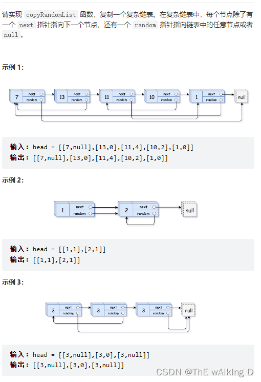
Sword finger offer 35 Replication of complex linked list
![[depth first search] 695 Maximum area of the island](/img/08/cfff4aec667216e4f146205a12c13f.jpg)
[depth first search] 695 Maximum area of the island
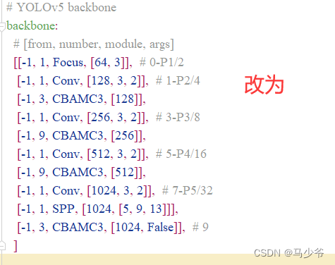
YOLOv5添加注意力机制
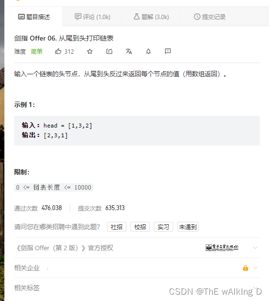
Sword finger offer 06 Print linked list from beginning to end

Double pointer Foundation

【实战技能】如何做好技术培训?
Fragment addition failed error lookup
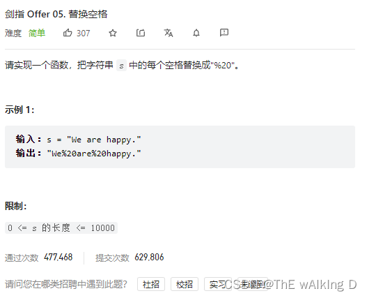
Sword finger offer 05 Replace spaces
![To be continued] [UE4 notes] L4 object editing](/img/0f/cfe788f07423222f9eed90f4cece7d.jpg)
To be continued] [UE4 notes] L4 object editing
随机推荐
Haut OJ 1352: string of choice
每日一题-无重复字符的最长子串
Developing desktop applications with electron
Pointnet++的改进
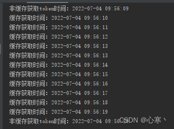
How can the Solon framework easily obtain the response time of each request?
【Jailhouse 文章】Look Mum, no VM Exits
Cluster script of data warehouse project
Sword finger offer 05 Replace spaces
Haut OJ 1221: a tired day
sync. Interpretation of mutex source code
游戏商城毕业设计
Graduation project of game mall
Detailed explanation of expression (csp-j 2021 expr) topic
剑指 Offer 35.复杂链表的复制
Solution to the palindrome string (Luogu p5041 haoi2009)
To be continued] [UE4 notes] L4 object editing
每日一题-搜索二维矩阵ps二维数组的查找
Time complexity and space complexity
Support multi-mode polymorphic gbase 8C database continuous innovation and heavy upgrade
[merge array] 88 merge two ordered arrays