[opencv learning] [common image convolution kernel]

Today, learn the influence of different styles of check images
It can be basically divided into high pass filtering and low-pass filtering
# Some low pass filters , Is to take the low-frequency components of the image , It's actually blurring the image / Gentle , Eliminate noise points , Such as the mean filter and Gaussian filter learned before .
# Some high pass filters , Is to take the high-frequency components of the image , In fact, it is to sharpen the image , Make the edge information of the image more prominent , Such as Sobel operator 、Prewitt operator 、 Sharpening filter, etc ;

The first part ： low pass filter

import cv2
import numpy as np


#  Show the image , Encapsulate as a function 
def cv_show_image(name, img):
    cv2.imshow(name, img)
    cv2.waitKey(0)  #  Waiting time , In milliseconds ,0 Represents any key termination 
    cv2.destroyAllWindows()



#  Some nuclear operations 
#  The first part ： Mean filter and Gaussian filter 
img = cv2.imread('images/saoge.jpg')  #  Read the original image 
img = cv2.resize(img, (0, 0), fx=0.5, fy=0.5)  #  The image is too big , Show smaller .
cv_show_image('img_src', img)

#  Define a 3x3 Mean kernel of , All weights are the same 
kernel = np.array([[1/9, 1/9, 1/9],
                   [1/9, 1/9, 1/9],
                   [1/9, 1/9, 1/9]], np.float32)
dst = cv2.filter2D(img, -1, kernel=kernel)
cv_show_image('mean_kernel', dst)

#  Define a 3x3 Gauss kernel of , The closer to the center, the heavier the weight , The further away from the center , The smaller the weight , The sampling of weights can be the sampling using normal distribution 
kernel = np.array([[1/16, 2/16, 1/16],
                   [2/16, 4/16, 2/16],
                   [1/16, 2/16, 1/16]], np.float32)
dst = cv2.filter2D(img, -1, kernel=kernel)
cv_show_image('gauss_kernel', dst)

Mean filtering results

Gaussian filtering result

The second part ： Sharpening filter

#  The second part ： Sharpen the image , Highlight the middle pixel , And suppress the surrounding pixels ,  Can be divided into 4- Adjacency sum 8 Adjacency 
#  for example  4- Adjacency 
# [[0, -1, 0],
# [-1, 5, -1],
# [ 0, -1, 0]]
#  for example  8- Adjacency 
# [[-1, -1, -1],
# [-1, 9, -1],
# [-1, -1, -1]]

kernel = np.array([[0, -1, 0], 
                   [-1, 4, -1], 
                   [0, -1, 0]], np.float32)  #  Define a 3x3 Sharpening nucleus of 
dst0 = cv2.filter2D(img, -1, kernel=kernel)
# cv_show_image('RuiHua', dst0)
kernel = np.array([[0, -1, 0], 
                   [-1, 5, -1], 
                   [0, -1, 0]], np.float32)  #  Define a 3x3 Sharpening nucleus of 
dst1 = cv2.filter2D(img, -1, kernel=kernel)
# cv_show_image('RuiHua', dst1)
kernel = np.array([[0, -1, 0], 
                   [-1, 6, -1], 
                   [0, -1, 0]], np.float32)  #  Define a 3x3 Sharpening nucleus of 
dst2 = cv2.filter2D(img, -1, kernel=kernel)
# cv_show_image('RuiHua', dst2)

res = np.vstack((dst0, dst1, dst2))  #  Display vertically 
cv2.imshow('Ruihua_k0_4', res)
cv2.waitKey(0)
cv2.destroyAllWindows()

kernel = np.array([[-1, -1, -1], 
                   [-1, 7, -1], 
                   [-1, -1, -1]], np.float32)  #  Define a 3x3 Sharpening nucleus of 
dst0 = cv2.filter2D(img, -1, kernel=kernel)
# cv_show_image('RuiHua', dst1)
kernel = np.array([[-1, -1, -1], 
                   [-1, 8, -1], 
                   [-1, -1, -1]], np.float32)  #  Define a 3x3 Sharpening nucleus of 
dst1 = cv2.filter2D(img, -1, kernel=kernel)
# cv_show_image('RuiHua', dst1)
kernel = np.array([[-1, -1, -1], 
                   [-1, 9, -1], 
                   [-1, -1, -1]], np.float32)  #  Define a 3x3 Sharpening nucleus of 
dst2 = cv2.filter2D(img, -1, kernel=kernel)
# cv_show_image('RuiHua', dst2)

res = np.hstack((dst0, dst1, dst2))  #  Display horizontally 
cv2.imshow('Ruihua_k1_8', res)
cv2.waitKey(0)
cv2.destroyAllWindows()

Varied 4 Adjacent nucleus sharpening effect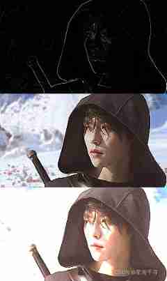

Varied 8 Adjacent nucleus sharpening effect

The third part ： First order differential kernel

#  The third part ： First order differential operators 
#  The edge of the object in the image is often the part that changes violently （ High frequency part ）, For a function , Where changes are more intense , The greater the absolute value of the corresponding derivative .
#  Image is a binary function ,f(x,y) Express (x,y) Value of pixels at ,
#  So the derivative is in addition to size , And direction . Then find the first derivative of the image in a certain direction （ Or gradient of image ）, It can also reflect the change degree of the image there , The faster the degree of change , In the vertical direction of this direction, there may be the edge of the object .
#  The first-order differential operator can calculate the edge of the object in a certain direction , But they are often sensitive to noise , And the sensitivity of edge detection depends on the size of the object .

# Prewitt operator 
# Prewitt The operator is to make a difference on the image to approximate the first derivative of a certain part of the image . Because the derivative also has directionality ,
#  So the same size Prewitt Operator and 8 Different types , The purpose is to seek 、 Next 、 Left 、 Right 、 Top left 、 The lower left 、 The upper right 、 The lower right 8 Gradient in two directions .
#  For example, the operator in the right gradient direction 
# [[-1, 0, 1],
# [-1, 0, 1],
# [-1, 0, 1]]
#  For example, the operator in the right up gradient direction 
# [[ 0, 1, 1],
# [-1, 0, 1],
# [-1, -1, 0]]
#  For example, the operator in the upward gradient direction 
# [[1, 1, 1],
# [0, 0, 1],
# [-1, -1, -1]]
#  For example, the operator in the upper left gradient direction 
# [[1, 1, 0],
# [1, 0, -1],
# [0, -1, -1]]
#  And so on 
kernel = np.array([[-1, -1, -1],
                   [0, 0, 0],
                   [1, 1, 1]], np.float32)  #  Define a 3x3 The convolution kernel of the downward gradient of 
dst_down = cv2.filter2D(img, -1, kernel=kernel)
# cv_show_image('RuiHua', dst0)
kernel = np.array([[-1, 0, 1],
                   [-1, 0, 1],
                   [-1, 0, 1]], np.float32)  #  Define a 3x3 Convolution kernel of right gradient 
dst_right = cv2.filter2D(img, -1, kernel=kernel)
# cv_show_image('RuiHua', dst0)
kernel = np.array([[1, 0, -1],
                   [1, 0, -1],
                   [1, 0, -1]], np.float32)  #  Define a 3x3 Convolution kernel of left gradient 
dst_left = cv2.filter2D(img, -1, kernel=kernel)
# cv_show_image('RuiHua', dst1)
kernel = np.array([[1, 1, 1],
                   [0, 0, 0],
                   [-1, -1, -1]], np.float32)  #  Define a 3x3 The convolution kernel of the upward gradient of 
dst_up = cv2.filter2D(img, -1, kernel=kernel)
# cv_show_image('RuiHua', dst2)

res = np.hstack((dst_down, dst_right, dst_left, dst_up))  #  Display vertically 
cv2.imshow('YiJie_Prewitt', res)
cv2.waitKey(0)
cv2.destroyAllWindows()

# sobel  operator 
# Sobel The operator is Prewitt An improved version of the operator , The middle elements are appropriately weighted ,Sobel Operator to Prewitt The operator is similar to Gaussian filtering and mean filtering .
#  Again Prewitt operator ,Sobel Consider the direction as an operator 
#  For example, the operator in the right gradient direction 
# [[-1, 0, 1],
# [-2, 0, 2],
# [-1, 0, 1]]
#  For example, the operator in the right up gradient direction 
# [[ 0, 1, 2],
# [-1, 0, 1],
# [-2, -1, 0]]
#  For example, the operator in the upward gradient direction 
# [[1, 2, 1],
# [0, 0, 1],
# [-1, -2, -1]]
#  For example, the operator in the upper left gradient direction 
# [[2, 1, 0],
# [1, 0, -1],
# [0, -1, -2]]
#  And so on 
kernel = np.array([[-1, -2, -1],
                   [0, 0, 0],
                   [1, 2, 1]], np.float32)  #  Define a 3x3 The convolution kernel of the downward gradient of 
dst_down = cv2.filter2D(img, -1, kernel=kernel)
# cv_show_image('RuiHua', dst0)
kernel = np.array([[-1, 0, 1],
                   [-2, 0, 2],
                   [-1, 0, 1]], np.float32)  #  Define a 3x3 Convolution kernel of right gradient 
dst_right = cv2.filter2D(img, -1, kernel=kernel)
# cv_show_image('RuiHua', dst0)
kernel = np.array([[1, 0, -1],
                   [2, 0, -2],
                   [1, 0, -1]], np.float32)  #  Define a 3x3 Convolution kernel of left gradient 
dst_left = cv2.filter2D(img, -1, kernel=kernel)
# cv_show_image('RuiHua', dst1)
kernel = np.array([[1, 2, 1],
                   [0, 0, 0],
                   [-1, -2, -1]], np.float32)  #  Define a 3x3 The convolution kernel of the upward gradient of 
dst_up = cv2.filter2D(img, -1, kernel=kernel)
# cv_show_image('RuiHua', dst2)

res = np.hstack((dst_down, dst_right, dst_left, dst_up))  #  Display vertically 
cv2.imshow('YiJie_sobel', res)
cv2.waitKey(0)
cv2.destroyAllWindows()

Varied Prewitt Operator effect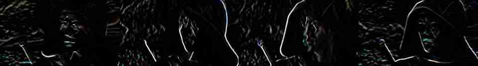

Varied Sobel Operator effect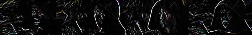

The fourth part ： Second order differential kernel

#  The fourth part ： Second order operator 
# Prewitt Operator and Sobel Operators are approximate to calculate the first derivative of the image , Only edges in a specific direction can be extracted .
#  The second derivative of a function is 0 when , Represents the extreme value of the first derivative here , Correspondingly, it shows that the original function changes the most here .
#  Therefore, it can often be based on the position of the zero crossing point of the second derivative of the image , To predict the most dramatic changes in the image , Maybe it corresponds to the edge of the object .
#  Different from the first-order differential operator , These second-order differential operators have rotation invariance for the calculation of edges , That is, edges in all directions can be detected .

# Laplace operator 
# Laplace The operator can approximately calculate the second derivative of the image , It has rotation invariance , That is, edges in all directions can be detected .
# Laplace There are two kinds of operators , Consider separately 4- Adjacency （D4） and 8- Adjacency （D8） Second order differential of two neighborhoods .
#  For example, one 3x3 Of 4- Adjacency is 
#  for example  4- Adjacency 
# [[0, -1, 0],
# [-1, 4, -1],
# [ 0, -1, 0]]
#  for example  8- Adjacency 
# [[-1, -1, -1],
# [ -1, 8, -1],
# [ -1, -1, -1]]
#
kernel = np.array([[0, -1, 0],
                   [-1, 4, -1],
                   [0, -1, 0]], np.float32)  #  Define a 3x3 Convolution kernel of left gradient 
dst1 = cv2.filter2D(img, -1, kernel=kernel)
# cv_show_image('RuiHua', dst1)
kernel = np.array([[-1, -1, -1],
                   [-1, 8, -1],
                   [-1, -1, -1]], np.float32)  #  Define a 3x3 The convolution kernel of the upward gradient of 
dst2 = cv2.filter2D(img, -1, kernel=kernel)
# cv_show_image('RuiHua', dst2)

res = np.hstack((dst1, dst2))  #  Display vertically 
cv2.imshow('ErJie_Laplace', res)
cv2.waitKey(0)
cv2.destroyAllWindows()


# LoG operator 
# Laplace Operators are still sensitive to noise . Therefore, Gaussian filter is often used to smooth the image first , Reuse Laplace Operators calculate second-order differential .
#  The combination of the two is called LoG operator （Laplacian of Gaussian）, This operator can calculate the second-order differential of image more stably .
#  For example, a commonly used 5x5 Its core is 
# [[0, 0, 1, 0, 0],
# [0, 1, 2, 1, 0],
# [1, 2, -16, 2, 1],
# [0, 1, 2, 1, 0],
# [0, 0, 1, 0, 0]]
kernel = np.array([[0, 0,  1, 0, 0],
                   [0, 1,  2,   1, 0],
                   [1, 2,  -17, 2, 1],
                   [0, 1,  2,   1, 0],
                   [0, 0,  1,   0, 0]], np.float32)  #  Define a 3x3 Convolution kernel of left gradient 
dst0 = cv2.filter2D(img, -1, kernel=kernel)
# cv_show_image('RuiHua', dst1)
kernel = np.array([[0, 0,  1, 0, 0],
                   [0, 1,  2,   1, 0],
                   [1, 2,  -16, 2, 1],
                   [0, 1,  2,   1, 0],
                   [0, 0,  1,   0, 0]], np.float32)  #  Define a 3x3 Convolution kernel of left gradient 
dst1 = cv2.filter2D(img, -1, kernel=kernel)
# cv_show_image('RuiHua', dst1)
kernel = np.array([[0, 0,  1, 0, 0],
                   [0, 1,  2,   1, 0],
                   [1, 2,  -15, 2, 1],
                   [0, 1,  2,   1, 0],
                   [0, 0,  1,   0, 0]], np.float32)  #  Define a 3x3 Convolution kernel of left gradient 
dst2 = cv2.filter2D(img, -1, kernel=kernel)
# cv_show_image('RuiHua', dst1)

res = np.hstack((dst0, dst1, dst2))  #  Display vertically 
cv2.imshow('ErJie_LoG', res)
cv2.waitKey(0)
cv2.destroyAllWindows()

Laplace Operator effect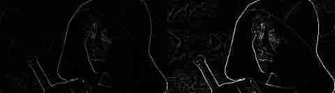

LoG operator