当前位置:网站首页>R language classification
R language classification
2022-07-03 10:23:00 【Small tear nevus of atobe】
R Problems encountered in language
wildcard
%*% Matrix multiplicationPCA Principal component analysis
#1 Import data
data(iris)# Import the built-in data set directly
head(iris)
#2 Centralize variables ( Subtract the mean value from each data ) And standardization ( And divide it by the standard deviation )
iris2=scale(iris[,1:4], center=T,scale=T)
head(iris2)
#3 Calculate the covariance matrix
cm1<-cor(iris2)
cm1
#4 Calculate the eigenvalue matrix , Get eigenvalues and eigenvectors
rs1<-eigen(cm1)
rs1
eigenvalues <- rs1$values
eigenvector2 <- as.matrix(rs1$vectors)
#5 Calculate the variance contribution of each variable
(Proportion_of_Variance <- eigenvalues/sum(eigenvalues))
(Cumulative_Proportion <- cumsum(Proportion_of_Variance))
# Drawing the gravel map
par(mar=c(6,6,2,2))
plot(rs1$values,type="b",
     cex=2,
     cex.lab=2,
     cex.axis=2,
     lty=2,
     lwd=2,
     xlab = "Principal components",
     ylab="Eigenvalues")
# Calculate the principal component score
dt<-as.matrix(iris2)
PC <- dt %*% eigenvector2
colnames(PC) <- c("PC1","PC2","PC3","PC4")
head(PC)
# Combine principal component scores and category labels
iris3<-data.frame(PC,iris$V5)
head(iris3)
# Calculate the variance contribution value of the first two principal components
xlab<-paste0("PC1(",round(Proportion_of_Variance[1]*100,2),"%)")
ylab<-paste0("PC2(",round(Proportion_of_Variance[2]*100,2),"%)")
# Draw the category matrix
p1<-ggplot(data = iris3,aes(x=PC1,y=PC2,color=iris3[,5]))+
  stat_ellipse(aes(fill=iris3[,5]),
               type ="norm", geom ="polygon",alpha=0.2,color=NA)+
  geom_point()+labs(x=xlab,y=ylab,color="")+
  guides(fill=F)
p1
- LDA discriminant analysis
And text mining LDA distinguish , Classification of LDA Model refers to projecting data into a discriminant equation , Make the inter class data variance as large as possible , The variance of intra class data should be as small as possible . The maximum number of discriminant equations is min( Number of categories of labels -1, The amount of data that needs to be predicted ), At the same time of classification, dimensionality reduction can also be achieved , The discriminant equation is the new dimension .
And the previous pca The difference in method is ,pca It is to eliminate variables that have little impact on category labels , And no category labels are required .
#LDA model
f <- paste(names(train_raw.df)[5], "~", paste(names(train_raw.df)[-5], collapse=" + "))# Build regression equation
iris_raw.lda <- lda(as.formula(paste(f)), data = train_raw.df)
iris_raw.lda.predict <- predict(iris_raw.lda, newdata = test_raw.df)
# Use LDA To make predictions
pred_y<-iris_raw.lda.predict$class
# draw LDA Prediction chart
ldaPreds <- iris_raw.lda.predict$x
head(ldaPreds)
test_raw.df %>%
  mutate(LD1 = ldaPreds[, 1],
         LD2 = ldaPreds[, 2]) %>%
  ggplot(aes(LD1, LD2, col = species)) +
  geom_point() +
  stat_ellipse() +
  theme_bw()
# According to the prediction , Calculate the prediction accuracy
t = table(pred_y,test_y)
acc1 = sum(diag(t))/nrow(test_x) *100
print(paste(" The accuracy of model prediction is :",round(acc1,4),'%',sep=''))
#ROC
lda_pre2 = predict(iris_raw.lda,test_raw.df,type = "prob")
roc_lda=multiclass.roc(test_y,lda_pre2$posterior)
auc(roc_lda)
- Decision tree
There are two kinds of regression tree and classification tree , call R In language rpart package . If it is a classification tree, you need to quantify the category label to identify , Subsequent calls predict Function prediction can be selected type yes prob still class, Then we can get the data of posterior probability , Calculation ROC Curve data .
#Decesion Tree
library(rpart)
library(rpart.plot)
library(caret)
train_raw.df$species <- factor(train_raw.df$species)# Category label vectorization
tree = rpart(species ~ .,data = train_raw.df)# Classification tree model
summary(tree)
rpart.plot(tree,type = 2)# Draw decision tree
tree_pre1 = predict(tree,test_raw.df) # Prediction accuracy
t2 = table(tree_pre1,test_y)
acc2 = sum(diag(t2))/nrow(test_x) *100
print(paste(" The accuracy of model prediction is :",round(acc2,4),'%',sep=''))
tree_pre2 = predict(tree,test_raw.df,type = "prob")
roc_tree=multiclass.roc(test_y, tree_pre2$posterior)
auc(roc_tree)
- Classification algorithm evaluation index
Multi classification algorithm calculation ROC(Receiver Operating characteristic Curve) Curve should call pROC Bag multiclass.roc function , Two classification algorithm can be used directly roc function . The multi classification algorithm uses computation roc Generally, you can only get AUC(Multi-class area under the curve) Value , namely ROC The area under the curve enclosed by the coordinate axis ,AUC The value range of is 0.5 and 1 Between .AUC The closer the 1.0, The better the prediction effect of the model ; be equal to 0.5 when , The authenticity is the lowest , No application value . If you want to draw ROC The graph should specify two classification labels .
边栏推荐
- Leetcode-106:根据中后序遍历序列构造二叉树
- Codeup: word replacement
- [LZY learning notes dive into deep learning] 3.1-3.3 principle and implementation of linear regression
- Implementation of "quick start electronic" window dragging
- [C question set] of Ⅵ
- 20220605数学:两数相除
- Hands on deep learning pytorch version exercise answer - 2.2 preliminary knowledge / data preprocessing
- MySQL root user needs sudo login
- 20220601 Mathematics: zero after factorial
- CV learning notes - deep learning
猜你喜欢

LeetCode - 1670 設計前中後隊列(設計 - 兩個雙端隊列)
![[C question set] of Ⅵ](/img/49/eb31cd26f7efbc4d57f17dc1321092.jpg)
[C question set] of Ⅵ

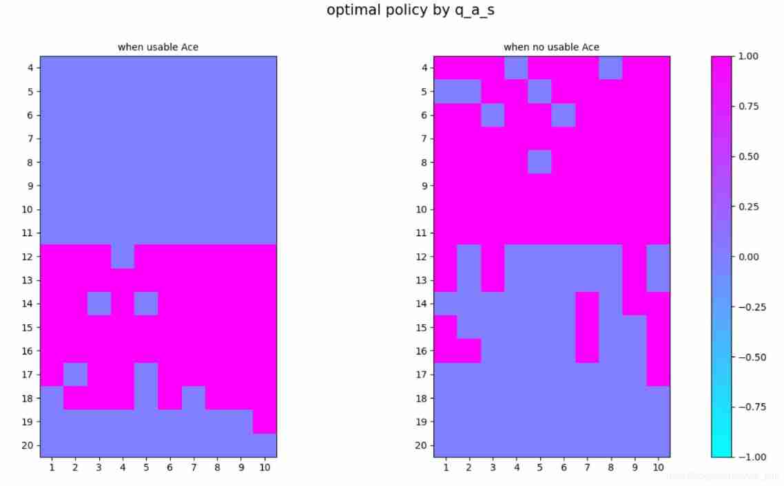
3.3 Monte Carlo Methods: case study: Blackjack of Policy Improvement of on- & off-policy Evaluation

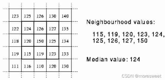
CV learning notes - image filter

Opencv image rotation

Leetcode interview question 17.20 Continuous median (large top pile + small top pile)

一步教你溯源【钓鱼邮件】的IP地址
![[LZY learning notes -dive into deep learning] math preparation 2.1-2.4](/img/92/955df4a810adff69a1c07208cb624e.jpg)
[LZY learning notes -dive into deep learning] math preparation 2.1-2.4

Policy gradient Method of Deep Reinforcement learning (Part One)

Leetcode-112: path sum
随机推荐
LeetCode - 895 最大频率栈(设计- 哈希表+优先队列 哈希表 + 栈) *
Advantageous distinctive domain adaptation reading notes (detailed)
Leetcode - 706 design hash mapping (Design)*
One click generate traffic password (exaggerated advertisement title)
LeetCode - 715. Range 模块(TreeSet) *****
LeetCode - 703 数据流中的第 K 大元素(设计 - 优先队列)
2018 Lenovo y7000 black apple external display scheme
Basic use and actual combat sharing of crash tool
20220604数学:x的平方根
20220602数学:Excel表列序号
Vgg16 migration learning source code
Opencv histogram equalization
[combinatorics] Introduction to Combinatorics (combinatorial idea 3: upper and lower bound approximation | upper and lower bound approximation example Remsey number)
Leetcode-100:相同的树
20220609 other: most elements
QT self drawing button with bubbles
Leetcode 300 longest ascending subsequence
CV learning notes - feature extraction
After clicking the Save button, you can only click it once
Leetcode - 5 longest palindrome substring