当前位置:网站首页>ML's shap: Based on the adult census income binary prediction data set (whether the predicted annual income exceeds 50K), use the shap decision diagram combined with the lightgbm model to realize the
ML's shap: Based on the adult census income binary prediction data set (whether the predicted annual income exceeds 50K), use the shap decision diagram combined with the lightgbm model to realize the
2022-07-07 05:58:00 【A Virgo procedural ape】
ML And shap: be based on adult Census income two classification forecast data set ( Whether the predicted annual income exceeds 50k) utilize shap Decision diagram combination LightGBM A detailed introduction to the case of outlier detection based on the model
Catalog
# 2.1、 Preliminary screening of modeling features
# 2.2、 Target feature binarization
# 2.3、 Category feature coding digitization
# 2.4、 Separate features from labels
#3、 Model training and reasoning
# 3.2、 Model building and training
# 4、 utilize shap Decision graph for outlier detection
# 4.1、 A small part of the original data and the preprocessed data are sampled respectively
# 4.2、 establish Explainer And calculate SHAP value
# 4.3、shap Visualization of decision diagram
Related articles
ML And shap: be based on adult Census income two classification forecast data set ( Whether the predicted annual income exceeds 50k) utilize shap Decision diagram combination LightGBM A detailed introduction to the case of outlier detection based on the model
ML And shap: be based on adult Census income two classification forecast data set ( Whether the predicted annual income exceeds 50k) utilize shap Decision diagram combination LightGBM Model implementation of outlier detection case detailed strategy implementation
be based on adult Census income two classification forecast data set ( Whether the predicted annual income exceeds 50k) utilize shap Decision diagram combination LightGBM A detailed introduction to the case of outlier detection based on the model
# 1、 Define datasets
| age | workclass | fnlwgt | education | education_num | marital_status | occupation | relationship | race | sex | capital_gain | capital_loss | hours_per_week | native_country | salary |
| 39 | State-gov | 77516 | Bachelors | 13 | Never-married | Adm-clerical | Not-in-family | White | Male | 2174 | 0 | 40 | United-States | <=50K |
| 50 | Self-emp-not-inc | 83311 | Bachelors | 13 | Married-civ-spouse | Exec-managerial | Husband | White | Male | 0 | 0 | 13 | United-States | <=50K |
| 38 | Private | 215646 | HS-grad | 9 | Divorced | Handlers-cleaners | Not-in-family | White | Male | 0 | 0 | 40 | United-States | <=50K |
| 53 | Private | 234721 | 11th | 7 | Married-civ-spouse | Handlers-cleaners | Husband | Black | Male | 0 | 0 | 40 | United-States | <=50K |
| 28 | Private | 338409 | Bachelors | 13 | Married-civ-spouse | Prof-specialty | Wife | Black | Female | 0 | 0 | 40 | Cuba | <=50K |
| 37 | Private | 284582 | Masters | 14 | Married-civ-spouse | Exec-managerial | Wife | White | Female | 0 | 0 | 40 | United-States | <=50K |
| 49 | Private | 160187 | 9th | 5 | Married-spouse-absent | Other-service | Not-in-family | Black | Female | 0 | 0 | 16 | Jamaica | <=50K |
| 52 | Self-emp-not-inc | 209642 | HS-grad | 9 | Married-civ-spouse | Exec-managerial | Husband | White | Male | 0 | 0 | 45 | United-States | >50K |
| 31 | Private | 45781 | Masters | 14 | Never-married | Prof-specialty | Not-in-family | White | Female | 14084 | 0 | 50 | United-States | >50K |
| 42 | Private | 159449 | Bachelors | 13 | Married-civ-spouse | Exec-managerial | Husband | White | Male | 5178 | 0 | 40 | United-States | >50K |
# 2、 Data set preprocessing
# 2.1、 Preliminary screening of modeling features
df.columns
14
# 2.2、 Target feature binarization
# 2.3、 Category feature coding digitization
| age | workclass | education_num | marital_status | occupation | relationship | race | sex | capital_gain | capital_loss | hours_per_week | native_country | salary | |
| 0 | 39 | 7 | 13 | 4 | 1 | 1 | 4 | 1 | 2174 | 0 | 40 | 39 | 0 |
| 1 | 50 | 6 | 13 | 2 | 4 | 0 | 4 | 1 | 0 | 0 | 13 | 39 | 0 |
| 2 | 38 | 4 | 9 | 0 | 6 | 1 | 4 | 1 | 0 | 0 | 40 | 39 | 0 |
| 3 | 53 | 4 | 7 | 2 | 6 | 0 | 2 | 1 | 0 | 0 | 40 | 39 | 0 |
| 4 | 28 | 4 | 13 | 2 | 10 | 5 | 2 | 0 | 0 | 0 | 40 | 5 | 0 |
| 5 | 37 | 4 | 14 | 2 | 4 | 5 | 4 | 0 | 0 | 0 | 40 | 39 | 0 |
| 6 | 49 | 4 | 5 | 3 | 8 | 1 | 2 | 0 | 0 | 0 | 16 | 23 | 0 |
| 7 | 52 | 6 | 9 | 2 | 4 | 0 | 4 | 1 | 0 | 0 | 45 | 39 | 1 |
| 8 | 31 | 4 | 14 | 4 | 10 | 1 | 4 | 0 | 14084 | 0 | 50 | 39 | 1 |
| 9 | 42 | 4 | 13 | 2 | 4 | 0 | 4 | 1 | 5178 | 0 | 40 | 39 | 1 |
# 2.4、 Separate features from labels
| age | workclass | education_num | marital_status | occupation | relationship | race | sex | capital_gain | capital_loss | hours_per_week | native_country |
| 39 | 7 | 13 | 4 | 1 | 1 | 4 | 1 | 2174 | 0 | 40 | 39 |
| 50 | 6 | 13 | 2 | 4 | 0 | 4 | 1 | 0 | 0 | 13 | 39 |
| 38 | 4 | 9 | 0 | 6 | 1 | 4 | 1 | 0 | 0 | 40 | 39 |
| 53 | 4 | 7 | 2 | 6 | 0 | 2 | 1 | 0 | 0 | 40 | 39 |
| 28 | 4 | 13 | 2 | 10 | 5 | 2 | 0 | 0 | 0 | 40 | 5 |
| 37 | 4 | 14 | 2 | 4 | 5 | 4 | 0 | 0 | 0 | 40 | 39 |
| 49 | 4 | 5 | 3 | 8 | 1 | 2 | 0 | 0 | 0 | 16 | 23 |
| 52 | 6 | 9 | 2 | 4 | 0 | 4 | 1 | 0 | 0 | 45 | 39 |
| 31 | 4 | 14 | 4 | 10 | 1 | 4 | 0 | 14084 | 0 | 50 | 39 |
| 42 | 4 | 13 | 2 | 4 | 0 | 4 | 1 | 5178 | 0 | 40 | 39 |
| salary |
| 0 |
| 0 |
| 0 |
| 0 |
| 0 |
| 0 |
| 0 |
| 1 |
| 1 |
| 1 |
#3、 Model training and reasoning
# 3.1、 Data set segmentation
X_test
| age | workclass | education_num | marital_status | occupation | relationship | race | sex | capital_gain | capital_loss | hours_per_week | native_country | |
| 1342 | 47 | 3 | 10 | 0 | 1 | 1 | 4 | 1 | 0 | 0 | 40 | 35 |
| 1338 | 71 | 3 | 13 | 0 | 13 | 3 | 4 | 0 | 2329 | 0 | 16 | 35 |
| 189 | 58 | 6 | 16 | 2 | 10 | 0 | 4 | 1 | 0 | 0 | 1 | 35 |
| 1332 | 23 | 3 | 9 | 4 | 7 | 1 | 2 | 1 | 0 | 0 | 35 | 35 |
| 1816 | 46 | 2 | 9 | 2 | 3 | 0 | 4 | 1 | 0 | 1902 | 40 | 35 |
| 1685 | 37 | 3 | 9 | 2 | 4 | 0 | 4 | 1 | 0 | 1902 | 45 | 35 |
| 657 | 34 | 3 | 9 | 2 | 3 | 0 | 4 | 1 | 0 | 0 | 45 | 35 |
| 1846 | 21 | 0 | 10 | 4 | 0 | 3 | 4 | 0 | 0 | 0 | 40 | 35 |
| 554 | 33 | 1 | 11 | 0 | 3 | 4 | 2 | 0 | 0 | 0 | 40 | 35 |
| 1963 | 49 | 3 | 13 | 2 | 12 | 0 | 4 | 1 | 0 | 0 | 50 | 35 |
# 3.2、 Model building and training
params = {
    "max_bin": 512, "learning_rate": 0.05,
    "boosting_type": "gbdt", "objective": "binary",
    "metric": "binary_logloss", "verbose": -1,
     "min_data": 100, "random_state": 1,
    "boost_from_average": True, "num_leaves": 10 }

LGBMC = lgb.train(params, lgbD_train, 10000,
                  valid_sets=[lgbD_test],
                  early_stopping_rounds=50,
                  verbose_eval=1000)
# 3.3、 Model to predict
| age | workclass | education_num | marital_status | occupation | relationship | race | sex | capital_gain | capital_loss | hours_per_week | native_country | y_test_predi | y_test | |
| 1342 | 47 | 3 | 10 | 0 | 1 | 1 | 4 | 1 | 0 | 0 | 40 | 35 | 0.045225575 | 0 |
| 1338 | 71 | 3 | 13 | 0 | 13 | 3 | 4 | 0 | 2329 | 0 | 16 | 35 | 0.074799172 | 0 |
| 189 | 58 | 6 | 16 | 2 | 10 | 0 | 4 | 1 | 0 | 0 | 1 | 35 | 0.30014332 | 1 |
| 1332 | 23 | 3 | 9 | 4 | 7 | 1 | 2 | 1 | 0 | 0 | 35 | 35 | 0.003966427 | 0 |
| 1816 | 46 | 2 | 9 | 2 | 3 | 0 | 4 | 1 | 0 | 1902 | 40 | 35 | 0.363861294 | 0 |
| 1685 | 37 | 3 | 9 | 2 | 4 | 0 | 4 | 1 | 0 | 1902 | 45 | 35 | 0.738628671 | 1 |
| 657 | 34 | 3 | 9 | 2 | 3 | 0 | 4 | 1 | 0 | 0 | 45 | 35 | 0.376412174 | 0 |
| 1846 | 21 | 0 | 10 | 4 | 0 | 3 | 4 | 0 | 0 | 0 | 40 | 35 | 0.002309884 | 0 |
| 554 | 33 | 1 | 11 | 0 | 3 | 4 | 2 | 0 | 0 | 0 | 40 | 35 | 0.060345836 | 1 |
| 1963 | 49 | 3 | 13 | 2 | 12 | 0 | 4 | 1 | 0 | 0 | 50 | 35 | 0.703506366 | 1 |
# 4、 utilize shap Decision graph for outlier detection
# 4.1、 A small part of the original data and the preprocessed data are sampled respectively
# 4.2、 establish Explainer And calculate SHAP value
shap2exp.values.shape (100, 12, 2)
[[[-5.97178729e-01 5.97178729e-01]
[-5.18879297e-03 5.18879297e-03]
[ 1.70566444e-01 -1.70566444e-01]
...
[ 0.00000000e+00 0.00000000e+00]
[ 6.58794799e-02 -6.58794799e-02]
[ 0.00000000e+00 0.00000000e+00]]
[[-4.45574118e-01 4.45574118e-01]
[-1.00665452e-03 1.00665452e-03]
[-8.12237233e-01 8.12237233e-01]
...
[ 0.00000000e+00 0.00000000e+00]
[ 8.56381961e-01 -8.56381961e-01]
[ 0.00000000e+00 0.00000000e+00]]
[[-3.87412165e-01 3.87412165e-01]
[ 1.52848351e-01 -1.52848351e-01]
[-1.02755954e+00 1.02755954e+00]
...
[ 0.00000000e+00 0.00000000e+00]
[ 1.10240434e+00 -1.10240434e+00]
[ 0.00000000e+00 0.00000000e+00]]
...
[[-5.28928223e-01 5.28928223e-01]
[ 7.14116015e-03 -7.14116015e-03]
[-8.82241728e-01 8.82241728e-01]
...
[ 0.00000000e+00 0.00000000e+00]
[ 7.47521189e-02 -7.47521189e-02]
[ 0.00000000e+00 0.00000000e+00]]
[[ 2.20002984e+00 -2.20002984e+00]
[ 7.75916086e-03 -7.75916086e-03]
[ 3.95152810e-01 -3.95152810e-01]
...
[ 0.00000000e+00 0.00000000e+00]
[ 1.52566789e-01 -1.52566789e-01]
[ 0.00000000e+00 0.00000000e+00]]
[[-8.28965461e-01 8.28965461e-01]
[-4.43687947e-02 4.43687947e-02]
[ 3.37305776e-01 -3.37305776e-01]
...
[ 0.00000000e+00 0.00000000e+00]
[ 8.26477289e-03 -8.26477289e-03]
[ 0.00000000e+00 0.00000000e+00]]]
shap2array.shape (100, 12)
LightGBM binary classifier with TreeExplainer shap values output has changed to a list of ndarray
[[ 5.97178729e-01 5.18879297e-03 -1.70566444e-01 ... 0.00000000e+00
-6.58794799e-02 0.00000000e+00]
[ 4.45574118e-01 1.00665452e-03 8.12237233e-01 ... 0.00000000e+00
-8.56381961e-01 0.00000000e+00]
[ 3.87412165e-01 -1.52848351e-01 1.02755954e+00 ... 0.00000000e+00
-1.10240434e+00 0.00000000e+00]
...
[ 5.28928223e-01 -7.14116015e-03 8.82241728e-01 ... 0.00000000e+00
-7.47521189e-02 0.00000000e+00]
[-2.20002984e+00 -7.75916086e-03 -3.95152810e-01 ... 0.00000000e+00
-1.52566789e-01 0.00000000e+00]
[ 8.28965461e-01 4.43687947e-02 -3.37305776e-01 ... 0.00000000e+00
-8.26477289e-03 0.00000000e+00]]
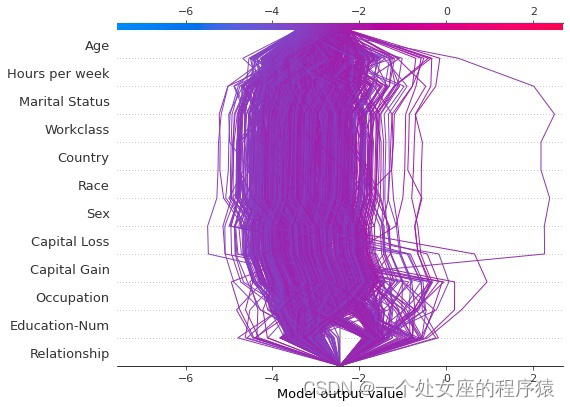
mode_exp_value: -1.9982244224656025# 4.3、shap Visualization of decision diagram
# Stacking the decision diagrams together helps shap Locate outliers , That is, the sample deviates from the dense group
边栏推荐
- An example of multi module collaboration based on NCF
- bat 批示处理详解
- Flask1.1.4 Werkzeug1.0.1 源碼分析:啟動流程
- 【SQL实战】一条SQL统计全国各地疫情分布情况
- 苹果cms V10模板/MXone Pro自适应影视电影网站模板
- 搞懂fastjson 对泛型的反序列化原理
- 线性回归
- 《HarmonyOS实战—入门到开发,浅析原子化服务》
- Classic questions about data storage
- 404 not found service cannot be reached in SAP WebService test
猜你喜欢
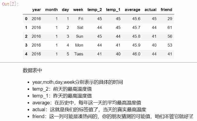
Pytorch builds neural network to predict temperature
Differences and introduction of cluster, distributed and microservice

Bat instruction processing details
每秒10W次分词搜索,产品经理又提了一个需求!!!(收藏)
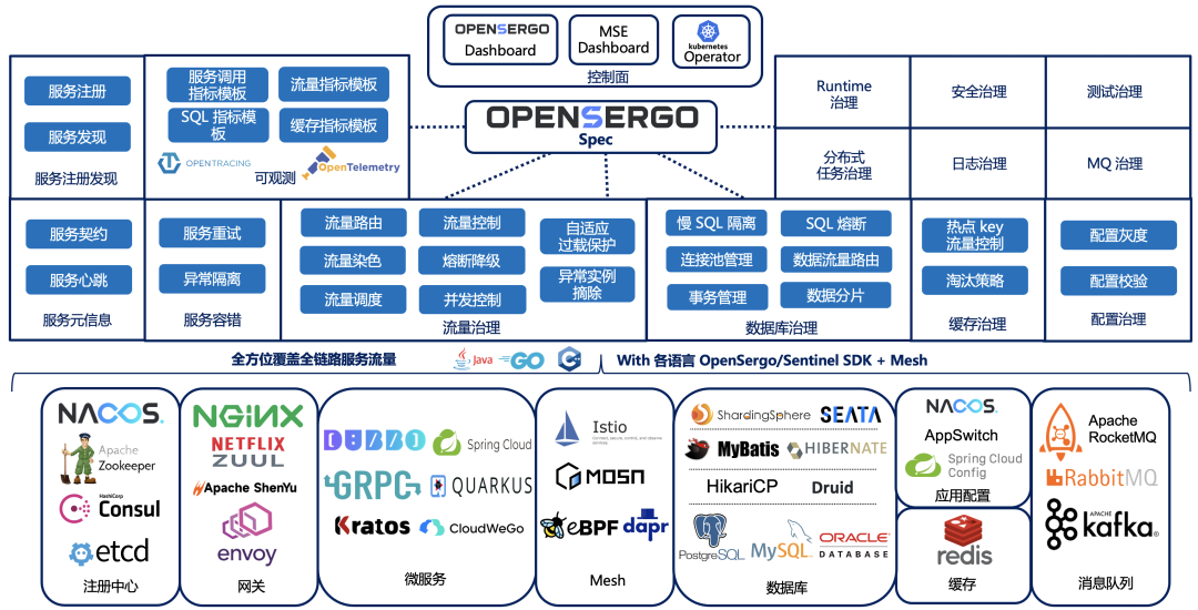
Opensergo is about to release v1alpha1, which will enrich the service governance capabilities of the full link heterogeneous architecture
Go语学习笔记 - gorm使用 - 原生sql、命名参数、Rows、ToSQL | Web框架Gin(九)
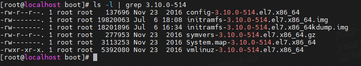
Red hat install kernel header file
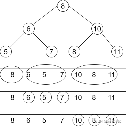
PTA ladder game exercise set l2-004 search tree judgment
cf:C. Column Swapping【排序 + 模擬】

pytorch_ 01 automatic derivation mechanism
随机推荐
Why does the data center need a set of infrastructure visual management system
如果不知道这4种缓存模式,敢说懂缓存吗?
Reading notes of Clickhouse principle analysis and Application Practice (6)
Flask1.1.4 werkzeug1.0.1 source code analysis: start the process
绕过open_basedir
PTA ladder game exercise set l2-004 search tree judgment
Sidecar mode
[云原生]微服务架构是什么?
Value range of various datetimes in SQL Server 2008
JVM命令之 jinfo:实时查看和修改JVM配置参数
Go language context explanation
《ClickHouse原理解析与应用实践》读书笔记(6)
Hcip eighth operation
SQL Server 2008 各种DateTime的取值范围
An example of multi module collaboration based on NCF
[cloud native] what is the microservice architecture?
【日常训练--腾讯精选50】292. Nim 游戏
[solved] record an error in easyexcel [when reading the XLS file, no error will be reported when reading the whole table, and an error will be reported when reading the specified sheet name]
async / await
980. Different path III DFS