当前位置:网站首页>[statistical learning method] learning notes - logistic regression and maximum entropy model
[statistical learning method] learning notes - logistic regression and maximum entropy model
2022-07-07 12:34:00 【Sickle leek】
Statistical learning methods learning notes —— Logistic regression and maximum entropy model
The return of logic (logistic regression) It is a classic classification method in statistical learning . Maximum entropy is a criterion for probabilistic model learning , It is extended to the classification problem to obtain the maximum entropy model (maximum entropy model). Logistic regression model and maximum entropy model belong to logarithmic linear model .
1. Logistic regression model
1.1 Logistic distribution (logistic distribution)
Definition ( Logistic distribution ) set up X obey continuity A random variable ,X Obeying the logistic distribution means X Have the following Distribution function and Density function :
F ( x ) = P ( X ≤ x ) = 1 1 + e − ( x − μ ) / r F(x)=P(X\le x)=\frac{1}{1+e^{-(x-\mu)/r}} F(x)=P(X≤x)=1+e−(x−μ)/r1
f ( x ) = F ′ ( x ) = e − ( x − μ ) / r γ ( 1 + e − ( x − μ ) / r ) 2 f(x)=F'(x)=\frac{e^{-(x-\mu)/r}}{\gamma (1+e^{-(x-\mu)/r})^2} f(x)=F′(x)=γ(1+e−(x−μ)/r)2e−(x−μ)/r
among , μ \mu μ For position parameters , γ > 0 \gamma >0 γ>0 For shape parameters .
Density function of logistic distribution f ( x ) f(x) f(x) And distribution function F ( x ) F(x) F(x) The figure of is shown in the figure below .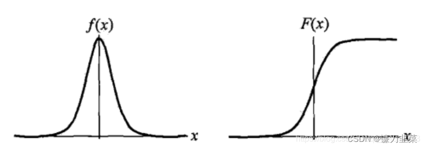
Distribution function belongs to logistic function , Its figure belongs to a S Shape curve (sigmoid curve). The curve is in point ( μ , 1 2 ) (\mu, \frac{1}{2}) (μ,21) It's central symmetry , The meet
F ( − x + μ ) − 1 2 = − F ( x + μ ) + 1 2 F(-x+\mu)-\frac{1}{2}=-F(x+\mu)+\frac{1}{2} F(−x+μ)−21=−F(x+μ)+21
The curve grows faster near the center , Slow growth at both ends . shape parameter γ \gamma γ The smaller the value of , The faster the curve grows near the center .
1.2 Binomial logistic regression (binomial logistic regression model)
Binomial logistic regression is a classification model , By conditional probability distribution P ( Y ∣ X ) P(Y|X) P(Y∣X) Express , In the form of parameterized logistic distribution . Here are random variables X The value is a real number , A random variable Y The value is 1 perhaps 0.
Definition ( Logistic regression model ): Binomial logistic regression model is the following conditional probability distribution :
P ( Y = 1 ∣ x ) = e x p ( w ⋅ x + b ) 1 + e x p ( w ⋅ x + b ) P(Y=1|x)=\frac{exp(w\cdot x + b)}{1+ exp(w\cdot x + b)} P(Y=1∣x)=1+exp(w⋅x+b)exp(w⋅x+b)
P ( Y = 0 ∣ x ) = 1 1 + e x p ( w ⋅ x + b ) P(Y=0|x)=\frac{1}{1+exp(w\cdot x +b)} P(Y=0∣x)=1+exp(w⋅x+b)1
here , x ∈ R n x\in R^n x∈Rn It's input , Y ∈ 0 , 1 Y\in {0, 1} Y∈0,1 It's output , w ∈ R n w\in R^n w∈Rn and b ∈ R b\in R b∈R Is the parameter , w call by power value towards The amount w It's called the weight vector w call by power value towards The amount , b b b For bias , w ⋅ x w\cdot x w⋅x by w and x Inner product .
Logistic regression compares two conditional probability values , Will instance x To the category with higher probability value .
Sometimes for convenience , The weight vector and input vector are extended , Still recorded as w,x namely w = ( w ( 1 ) , w ( 2 ) , . . . , w ( n ) , b ) T , x = ( x ( 1 ) , x ( 2 ) , . . . , x ( n ) , 1 ) T w=(w^{(1)}, w^{(2)}, ...,w^{(n)}, b)^T, x=(x^{(1)},x^{(2)},...,x^{(n)}, 1)^T w=(w(1),w(2),...,w(n),b)T,x=(x(1),x(2),...,x(n),1)T, be :
P ( Y = 1 ∣ x ) = e x p ( w ⋅ x ) 1 + e x p ( w ⋅ x ) P(Y=1|x)=\frac{exp(w\cdot x)}{1+ exp(w\cdot x)} P(Y=1∣x)=1+exp(w⋅x)exp(w⋅x)
P ( Y = 0 ∣ x ) = 1 1 + e x p ( w ⋅ x ) P(Y=0|x)=\frac{1}{1+exp(w\cdot x)} P(Y=0∣x)=1+exp(w⋅x)1
The characteristics of logistic regression . The probability of an event (odds) It refers to the ratio of the probability of the event occurring to the probability of the event not occurring . If the probability of the event is p, Then the probability of this event is p 1 − p \frac{p}{1-p} 1−pp, The logarithmic probability of the event (log odds) or logit The function is :
l o g i t ( p ) = l o g p 1 − p logit(p)=log \frac{p}{1-p} logit(p)=log1−pp
For logistic regression , Available :
l o g P ( Y = 1 ∣ x ) 1 − P ( Y = 1 ∣ x ) = w ⋅ x log\frac{P(Y=1|x)}{1- P(Y=1|x)}=w\cdot x log1−P(Y=1∣x)P(Y=1∣x)=w⋅x
That is to say , In the logistic regression model , Output Y=1 The logarithmic probability of is the input x The linear function of . Or say , Output Y=1 The logarithmic probability of is determined by the input x A model represented by a linear function , Logistic regression model . The closer the value of a linear function approaches positive infinity , The probability value is close to 1; The closer the value of a linear function is to negative infinity , The closer the probability value is to 0.
1.3 Estimation of model parameters
For a given set of training data T = { ( x 1 , y 1 ) , ( x 2 , y 2 ) , . . . , ( x N , y N ) } T=\{(x_1,y_1),(x_2,y_2),...,(x_N,y_N)\} T={ (x1,y1),(x2,y2),...,(xN,yN)}, among x i ∈ R n , y i ∈ { 0 , 1 } x_i\in R^n, y_i \in \{0,1\} xi∈Rn,yi∈{ 0,1}, The maximum likelihood estimation method can be used to estimate the model parameters , So we can get logistic regression model .
set up : P ( Y = 1 ∣ x ) = π ( x ) P(Y=1|x)=\pi (x) P(Y=1∣x)=π(x), P ( Y = 0 ∣ x ) = 1 − π ( x ) P(Y=0|x)=1-\pi (x) P(Y=0∣x)=1−π(x), The likelihood function is :
∏ i = 1 N [ π ( x i ) ] y i [ 1 − π ( x i ) ] 1 − y i \prod_{i=1}^N [\pi (x_i)]^{y_i}[1- \pi (x_i)]^{1-y_i} i=1∏N[π(xi)]yi[1−π(xi)]1−yi
The log likelihood function is :
L ( w ) = ∑ i = 1 N [ y i ( w ⋅ x i ) − log ( 1 + e x p ( w ⋅ x i ) ) ] L(w)=\sum_{i=1}^N [y_i(w\cdot x_i)-\log (1+exp(w\cdot x_i))] L(w)=i=1∑N[yi(w⋅xi)−log(1+exp(w⋅xi))]
Yes L ( w ) L(w) L(w) Find the maximum , obtain w The estimate of .
In this way, the problem becomes an optimization problem with log likelihood function as the objective function . The commonly used methods in logistic regression learning are gradient descent method and quasi Newton method .
hypothesis w w w The maximum likelihood estimate of is w ^ \hat {w} w^, Then the learned logistic regression model is :
P ( Y = 1 ∣ x ) = e x p ( w ^ ⋅ x ) 1 + e x p ( w ^ ⋅ x ) P(Y=1|x)=\frac{exp(\hat {w}\cdot x)}{1+ exp(\hat {w}\cdot x)} P(Y=1∣x)=1+exp(w^⋅x)exp(w^⋅x)
P ( Y = 0 ∣ x ) = 1 1 + e x p ( w ^ ⋅ x ) P(Y=0|x)=\frac{1}{1+exp(\hat {w}\cdot x)} P(Y=0∣x)=1+exp(w^⋅x)1
1.4 Multiple logistic regression (multi-nominal logistic regression model)
Suppose a discrete random variable Y The set of values for is {1,2,…, K}, So the multiple logistic regression model is :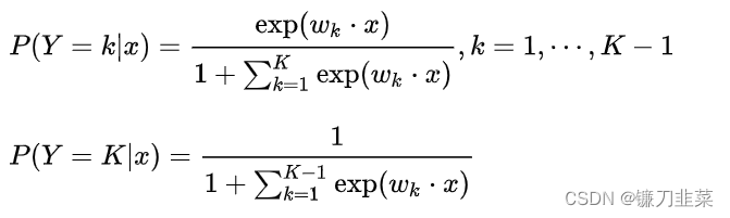
2. Maximum entropy model (maximum entropy model)
The maximum entropy model is derived from the principle of maximum entropy .
2.1 The principle of maximum entropy
The maximum entropy principle is a criterion for probabilistic model learning . Think , When learning probability models , In all possible probability models ( Distribution ) in , The model with the largest entropy is the best model . The set of probabilistic models is usually determined by constraints . therefore , The maximum entropy principle can also be described as selecting the model with the maximum entropy from the set of models that meet the constraints .
Then why choose maximum entropy ? Because without knowing any information , We can only assume that the data is relatively average in all values , That is, the degree of chaos is the greatest .
Assumed discrete random variable X The probability distribution of P ( X ) P(X) P(X), Then its entropy is
H ( P ) = − ∑ x P ( x ) l o g ( x ) H(P)=-\sum_x P(x)log (x) H(P)=−x∑P(x)log(x)
Entropy satisfies the following inequality :
0 ≤ H ( P ) ≤ log ∣ X ∣ 0 \le H(P) \le \log{|X|} 0≤H(P)≤log∣X∣
among , ∣ X ∣ |X| ∣X∣ yes X The number of values , If and only if X The equal sign on the right holds when the distribution of is uniform , That is to say, when X When the distribution is uniform , Entropy is maximum .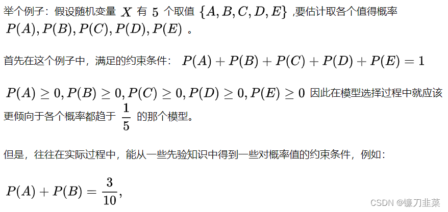
With this constraint , In the absence of other information ,, It can be said that A and B It's equal probability ,C、D and E It's equal probability , therefore :
P ( A ) = P ( B ) = 3 20 P(A)=P(B)=\frac{3}{20} P(A)=P(B)=203
P ( C ) = P ( D ) = P ( E ) = 7 20 P(C)=P(D)=P(E)=\frac{7}{20} P(C)=P(D)=P(E)=207
2.2 The definition of the maximum entropy model
Suppose the classification model is a conditional probability distribution P ( Y ∣ X ) P(Y|X) P(Y∣X), X ∈ X ∈ R n X\in\mathcal X\in\bold R^n X∈X∈Rn Indicates input , Y ∈ Y Y\in\mathcal Y Y∈Y Indicative output , X \mathcal X X and Y \mathcal Y Y Are the set of input and output respectively . This model represents for a given input X X X, With conditional probability P ( Y ∣ X ) P(Y|X) P(Y∣X) Output Y Y Y. Given a training data set T = { ( x 1 , y 1 ) , ( x 2 , y 2 ) , . . . , ( x N , y N ) } T=\{(x_1,y_1),(x_2 ,y_2),...,(x_N,y_N)\} T={ (x1,y1),(x2,y2),...,(xN,yN)}, The goal of learning is to use the maximum entropy principle to select the best classification model .
Given the training data set , We can determine the joint distribution P ( X , Y ) P(X,Y) P(X,Y) Empirical distribution and marginal distribution P ( X ) P(X) P(X) The distribution of experience , Respectively by P ~ ( X , Y ) {\tilde P}(X,Y) P~(X,Y) and P ~ ( X ) {\tilde P}(X) P~(X) Express :
P ~ ( X = x , Y = y ) = ν ( X = x , Y = y ) N {\tilde P}(X=x,Y=y)=\frac{\nu(X=x,Y=y)}{N} P~(X=x,Y=y)=Nν(X=x,Y=y)
P ~ ( X = x ) = ν ( X = x ) N {\tilde P}(X=x)=\frac{\nu(X=x)}{N} P~(X=x)=Nν(X=x)
In style ν ( X = x , Y = y ) \nu(X=x,Y=y) ν(X=x,Y=y) Represents the sample in the training data ( x , y ) (x,y) (x,y) Frequency of occurrence , ν ( X = x ) \nu(X=x) ν(X=x) Indicates input during training x x x Frequency of occurrence ,N Represents the training sample size . Then use a characteristic function (feature function) f ( x , y ) f(x,y) f(x,y) Description input x x x And the output y y y A fact between . Its definition is :
f ( x , y ) = { 1 , x and y full foot some One things real 0 , no be f(x,y)=\left\{\begin{matrix} 1, & x and y Satisfy a fact \\ 0, & otherwise \end{matrix}\right. f(x,y)={ 1,0,x and y full foot some One things real no be
The characteristic function f ( x , y ) f(x,y) f(x,y) About the distribution of experience P ~ ( X , Y ) {\tilde P}(X,Y) P~(X,Y) The expectation of :
E P ~ ( f ) = ∑ x , y P ~ ( x , y ) f ( x , y ) E_{\tilde P}(f)=\sum_{x,y}{\tilde P}(x,y)f(x,y) EP~(f)=x,y∑P~(x,y)f(x,y)
The characteristic function f ( x , y ) f(x,y) f(x,y) About the model P ( Y ∣ X ) P(Y|X) P(Y∣X) And experience distribution P ~ ( X , Y ) {\tilde P}(X,Y) P~(X,Y) The expectation of :
E P ( f ) = ∑ x , y P ~ ( x ) P ( y ∣ x ) f ( x , y ) E_P(f)=\sum_{x,y}{\tilde P}(x)P(y|x)f(x,y) EP(f)=x,y∑P~(x)P(y∣x)f(x,y)
If the model can get the information in training , Then we can assume that the two expectations are equal , namely :
E P ~ ( f ) = E P ( f ) E_{\tilde P}(f)=E_P(f) EP~(f)=EP(f)
namely :
∑ x , y P ~ ( x , y ) f ( x , y ) = ∑ x , y P ~ ( x ) P ( y ∣ x ) f ( x , y ) \sum_{x,y}{\tilde P}(x,y)f(x,y)=\sum_{x,y}{\tilde P}(x)P(y|x)f(x,y) x,y∑P~(x,y)f(x,y)=x,y∑P~(x)P(y∣x)f(x,y)
The above formula is the constraint condition of model learning .
Maximum entropy model Suppose that the set of models satisfying all the constraints is :
C = { P ∈ P ∣ E P ( f i ) = E P ~ ( f i ) , i = 1 , 2 , . . . , n } \mathcal C=\{P\in\mathcal P|E_{P}(f_i)=E_{\tilde P}(f_i),\ i=1,2,...,n\} C={ P∈P∣EP(fi)=EP~(fi), i=1,2,...,n}
Defined in conditional probability distribution P ( Y ∣ X ) P(Y|X) P(Y∣X) The conditional entropy on is :
H ( P ) = − ∑ x , y P ~ ( x ) P ( y ∣ x ) log P ( y ∣ x ) H(P)=-\sum_{x,y}{\tilde P}(x)P(y|x)\log P(y|x) H(P)=−x,y∑P~(x)P(y∣x)logP(y∣x)
Then the model set C \mathcal C C Medium conditional entropy H ( P ) H(P) H(P) The largest model is called the maximum entropy model .
2.3 Learning the maximum entropy model
The learning process of the maximum entropy model is The process of solving the maximum entropy model , It can also be formalized as a constrained optimization problem . Given the training data set T = { ( x 1 , y 1 ) , ( x 2 , y 2 ) , . . . , ( x N , y N ) } T=\{(x_1,y_1),(x_2,y_2),...,(x_N,y_N)\} T={ (x1,y1),(x2,y2),...,(xN,yN)} And the characteristic function f i ( x , y ) , i = 1 , 2 , . . . n f_i(x,y),\ i=1,2,...n fi(x,y), i=1,2,...n, The learning of the maximum entropy model is equivalent to the constrained optimization problem :
max P ∈ C H ( P ) = − ∑ x , y P ~ ( x ) P ( y ∣ x ) log P ( y ∣ x ) \max_{P\in\mathcal C}\ H(P)=-\sum_{x,y}\tilde P(x)P(y|x)\log P(y|x) P∈Cmax H(P)=−x,y∑P~(x)P(y∣x)logP(y∣x)
s . t . E P ( f i ) = E P ~ ( f i ) , i = 1 , 2 , . . . , n ∑ y P ( y ∣ x ) = 1 s.t.\ E_P(f_i)=E_{\tilde P}(f_i),\ i=1,2,...,n\ \ \ \sum_{y}P(y|x)=1 s.t. EP(fi)=EP~(fi), i=1,2,...,n y∑P(y∣x)=1
According to the habit of optimization problems , We Transform the problem of finding the maximum value into an equivalent problem of finding the minimum value :
min P ∈ C − H ( P ) = ∑ x , y P ~ ( x ) P ( y ∣ x ) log P ( y ∣ x ) \min_{P\in\mathcal C}\ -H(P)=\sum_{x,y}\tilde P(x)P(y|x)\log P(y|x) P∈Cmin −H(P)=x,y∑P~(x)P(y∣x)logP(y∣x)
s . t . E P ( f i ) = E P ~ ( f i ) , i = 1 , 2 , . . . , n ∑ y P ( y ∣ x ) = 1 s.t.\ E_P(f_i)=E_{\tilde P}(f_i),\ i=1,2,...,n\ \ \ \sum_{y}P(y|x)=1 s.t. EP(fi)=EP~(fi), i=1,2,...,n y∑P(y∣x)=1
here , The original problem of constrained optimization is transformed into the dual problem of unconstrained optimization . Solve the original problem by solving the dual problem .
For the above optimization problem , First , Introduce Lagrange multipliers w 0 , w 1 , . . . , w n w_0,w_1,...,w_n w0,w1,...,wn, Define the Lagrange function L ( P , w ) L(P,w) L(P,w):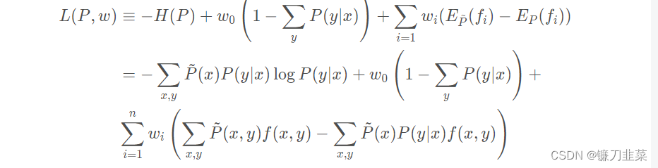
The original problem of optimization is :
min P ∈ C max w L ( P , w ) \min_{P\in \bold C}\max_wL(P,w) P∈CminwmaxL(P,w)
The dual problem is :
max w min P ∈ C L ( P , w ) \max_w\min_{P\in \bold C}L(P,w) wmaxP∈CminL(P,w)
Because of the Lagrange function L ( P , w ) L(P,w) L(P,w) yes P The convex function of , The solution of the primal problem is equivalent to the solution of the dual problem . In this way, the original problem can be solved by solving the dual problem .
First, solve the internal minimization problem min P ∈ C L ( P , w ) \min \limits_{P\in\bold C}L(P,w) P∈CminL(P,w), Write it down as :
Ψ ( w ) = min P ∈ C L ( P , w ) = L ( P w , w ) \Psi(w)=\min_{P\in\bold C}L(P,w)=L(P_w,w) Ψ(w)=P∈CminL(P,w)=L(Pw,w)
Ψ ( w ) \Psi(w) Ψ(w) It's called a dual function . meanwhile , Put it down as :
P w = arg min P ∈ C L ( P , w ) = P w ( y ∣ x ) P_w=\arg \min_{P\in\bold C}L(P,w)=P_w(y|x) Pw=argP∈CminL(P,w)=Pw(y∣x)
Then seek L ( P , w ) L(P,w) L(P,w) Yes P ( y ∣ x ) P(y|x) P(y∣x) Partial derivative of :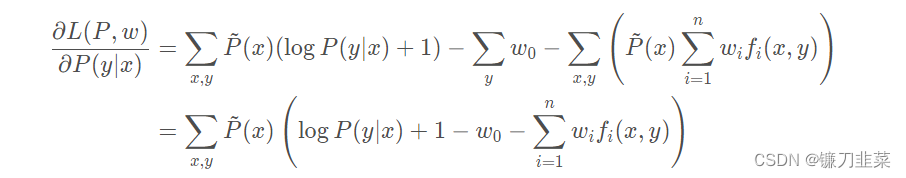
Let the partial derivative be equal to 0 And in P ~ ( x ) > 0 \tilde P(x)>0 P~(x)>0 Under the circumstances , Solution :
P ( y ∣ x ) = exp ( ∑ i = 1 n w i f i ( x , y ) + w 0 − 1 ) = exp ( ∑ i = 1 n w i f i ( x , y ) ) exp ( 1 − w 0 ) P(y|x)=\exp\left(\sum_{i=1}^nw_if_i(x,y)+w_0-1\right)=\frac{\exp\left(\sum \limits_{i=1}^nw_if_i(x,y)\right)}{\exp(1-w_0)} P(y∣x)=exp(i=1∑nwifi(x,y)+w0−1)=exp(1−w0)exp(i=1∑nwifi(x,y))
Due to constraints ∑ y P ( y ∣ x ) = 1 \sum \limits_{y}P(y|x)=1 y∑P(y∣x)=1, have to ( Here is based on and 1 Replace the denominator in the above formula with ):
P w ( y ∣ x ) = 1 Z w ( x ) exp ( ∑ i = 1 n w i f i ( x , y ) ) P_w(y|x)=\frac{1}{Z_w(x)}\exp\left(\sum_{i=1}^nw_if_i(x,y)\right) Pw(y∣x)=Zw(x)1exp(i=1∑nwifi(x,y))
among :
Z w ( x ) = ∑ y exp ( ∑ i = 1 n w i f i ( x , y ) ) Z_w(x)=\sum_{y}\exp\left(\sum_{i=1}^nw_if_i(x,y)\right) Zw(x)=y∑exp(i=1∑nwifi(x,y))
Z w ( x ) Z_w(x) Zw(x) It's called normalization factor ; f i ( x , y ) f_i(x,y) fi(x,y) It's a characteristic function ; w i w_i wi It's the weight of the feature .
after , Solve the maximization problem outside the dual problem :
max w Ψ ( w ) \max_w\Psi(w) maxwΨ(w)
Put it down as w ∗ w^* w∗, namely :
w ∗ = arg min w Ψ ( w ) w^*=\arg\min_w\Psi(w) w∗=argminwΨ(w)
2.3 Maximum likelihood estimation
The maximization of dual function is equivalent to the maximum likelihood estimation of maximum entropy model . Prove slightly .
The maximum entropy model has a similar form to the logistic regression model , They are also called log linear models (log linear model). Model learning is the maximum likelihood estimation or regularized maximum likelihood estimation of the model under the given training data conditions .
3. Optimization algorithms for model learning
Logistic regression model 、 The learning of maximum entropy model is reduced to the optimization problem with likelihood function as the objective function , Usually by iterative algorithm solve . At this time, the objective function is smooth Convex function , Common methods have improved Iterative scaling 、 Gradient descent method 、 Newton method and Quasi Newton method etc. . Newton method or quasi Newton method generally converges faster .
3.1 The improved iterative scaling method (improved iterative scaling, IIS)
IIS It is an optimization algorithm for maximum entropy model learning . The known maximum entropy model is :
P w ( y ∣ x ) = 1 Z w ( x ) exp ( ∑ i = 1 n w i f i ( x , y ) ) P_w(y|x)=\frac{1}{Z_w(x)}\exp\left(\sum_{i=1}^nw_if_i(x,y)\right) Pw(y∣x)=Zw(x)1exp(i=1∑nwifi(x,y))
among :
Z w ( x ) = ∑ y exp ( ∑ i = 1 n w i f i ( x , y ) ) Z_w(x)=\sum_{y}\exp\left(\sum_{i=1}^nw_if_i(x,y)\right) Zw(x)=y∑exp(i=1∑nwifi(x,y))
The log likelihood function is ( Derivation is omitted here ):
∑ x , y P ~ ( x , y ) ∑ i = 1 n w i f i ( x , y ) − ∑ x P ~ ( x ) log Z w ( x ) \sum_{x,y}\tilde P(x,y)\sum_{i=1}^nw_if_i(x,y)-\sum_x\tilde P(x)\log Z_w(x) x,y∑P~(x,y)i=1∑nwifi(x,y)−x∑P~(x)logZw(x)
The goal is to learn model parameters by maximum likelihood estimation , That is to find the maximum of the log likelihood function w ^ \hat w w^. The idea of the improved iterative scaling method is :== Suppose that the current parameter vector of the maximum entropy model is w = ( w 1 , w 2 , . . . , w n ) T w=(w_1,w_2,...,w_n)^{\rm T} w=(w1,w2,...,wn)T, We want to find a new parameter vector w + δ = ( w 1 + δ , w 2 + δ , . . . , w n + δ ) T w+\delta=(w_1+\delta,w_2+\delta,...,w_n+\delta)^{\rm T} w+δ=(w1+δ,w2+δ,...,wn+δ)T, Make the log likelihood function of the model increase . If there is such a method of updating parameter vectors τ : w → w + δ \tau: w\rightarrow w+\delta τ:w→w+δ, Then you can reuse this method , Until the maximum value of the log likelihood function is found . For a given empirical distribution P ~ ( x , y ) \tilde P(x,y) P~(x,y), Model parameters from w w w To w + δ w+\delta w+δ, The variable of log likelihood function is :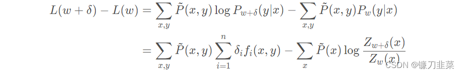
Using inequality :
− l o g α ≥ 1 − α , α > 0 −logα≥1−α, α>0 −logα≥1−α,α>0
Establish the lower bound of the variable of the log likelihood function :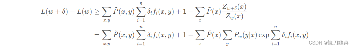
Mark the right end of the above formula as A ( δ ∣ w ) A(\delta|w) A(δ∣w), namely :
L ( w + δ ) − L ( w ) ≥ A ( δ ∣ w ) L(w+\delta)-L(w)\geq A(\delta|w) L(w+δ)−L(w)≥A(δ∣w)
namely A ( δ ∣ w ) A(\delta|w) A(δ∣w) Is a lower bound of the variable of the log likelihood function . If you can find the right δ \delta δ Raise the lower bound , Then the log likelihood function will also improve . However , function A ( δ ∣ w ) A(\delta|w) A(δ∣w) Medium δ \delta δ It's a vector , Contains multiple variables , Not easy to optimize at the same time . The improved iterative scaling method attempts to optimize only one of the variables δ i \delta_i δi, And fix other variables δ j , i ≠ j \delta_j, i\ne j δj,i=j.
For this purpose , The improved iterative scaling method further reduces the lower bound . In particular , Introduce a quantity f # ( x , y ) f^\#(x,y) f#(x,y):
f # ( x , y ) = ∑ i f i ( x , y ) f^\#(x,y)=\sum_if_i(x,y) f#(x,y)=i∑fi(x,y)
because f i f_i fi Is a binary function , so f # ( x , y ) f^\#(x,y) f#(x,y) Indicates that all features are in ( x , y ) (x,y) (x,y) Number of occurrences . such , A ( δ ∣ w ) A(\delta|w) A(δ∣w) to :
A ( δ ∣ w ) = ∑ x , y P ~ ( x , y ) ∑ i = 1 n δ i f i ( x , y ) + 1 − ∑ x P ~ ( x ) ∑ y P w ( y ∣ x ) exp ( f # ( x , y ) ∑ i = 1 n δ i f i ( x , y ) f # ( x , y ) ) (12) A(\delta|w)=\sum_{x,y}\tilde P(x,y)\sum_{i=1}^n\delta_if_i(x,y)+1-\sum_x\tilde P(x)\sum_yP_w(y|x)\exp\left(f^\#(x,y)\sum_{i=1}^n\frac{\delta_if_i(x,y)}{f^\#(x,y)}\right)\tag{12} A(δ∣w)=x,y∑P~(x,y)i=1∑nδifi(x,y)+1−x∑P~(x)y∑Pw(y∣x)exp(f#(x,y)i=1∑nf#(x,y)δifi(x,y))(12)
According to the definition , f i ( x , y ) f_i(x,y) fi(x,y) It means the first one i i i Characteristic in ( x , y ) (x,y) (x,y) Number of occurrences ; f # ( x , y ) f^\#(x,y) f#(x,y) Indicates that all features are in ( x , y ) (x,y) (x,y) Number of occurrences . So there is :
f i ( x , y ) f # ( x , y ) ≥ 0 , ∑ i = 1 n f i ( x , y ) f # ( x , y ) = 1 \frac{f_i(x,y)}{f^\#(x,y)}\geq0,\ \sum_{i=1}^n\frac{f_i(x,y)}{f^\#(x,y)}=1 f#(x,y)fi(x,y)≥0, i=1∑nf#(x,y)fi(x,y)=1
according to Jensen inequality :
f ( λ i ∑ i = 1 n f ( x i ) ≤ ∑ i = 1 n λ i f ( x i ) ) f\left(\lambda_i\sum \limits_{i=1}^nf(x_i)\leq\sum \limits_{i=1}^n\lambda_if(x_i)\right) f(λii=1∑nf(xi)≤i=1∑nλif(xi))
So there is :
exp ( ∑ i = 1 n f i ( x , y ) f # ( x , y ) δ i f # ( x , y ) ) ≤ ∑ i = 1 n f i ( x , y ) f # ( x , y ) exp ( δ i f # ( x , y ) ) \exp\left(\sum_{i=1}^n\frac{f_i(x,y)}{f^\#(x,y)}\delta_i{f^\#(x,y)}\right)\leq\sum_{i=1}^n\frac{f_i(x,y)}{f^\#(x,y)}\exp\left(\delta_if^\#(x,y)\right) exp(i=1∑nf#(x,y)fi(x,y)δif#(x,y))≤i=1∑nf#(x,y)fi(x,y)exp(δif#(x,y))
thus , type (11) I could rewrite it as :
A ( δ ∣ w ) ≥ ∑ x , y P ~ ( x , y ) ∑ i = 1 n δ i f i ( x , y ) + 1 − ∑ x P ~ ( x ) ∑ y P w ( y ∣ x ) ∑ i = 1 n f i ( x , y ) f # ( x , y ) exp ( δ i f # ( x , y ) ) A(\delta|w)\geq\sum_{x,y}\tilde P(x,y)\sum_{i=1}^n\delta_if_i(x,y)+1-\sum_x\tilde P(x)\sum_yP_w(y|x)\sum_{i=1}^n\frac{f_i(x,y)}{f^\#(x,y)}\exp\left(\delta_if^\#(x,y)\right) A(δ∣w)≥x,y∑P~(x,y)i=1∑nδifi(x,y)+1−x∑P~(x)y∑Pw(y∣x)i=1∑nf#(x,y)fi(x,y)exp(δif#(x,y))
Remember that the right end of the equation is B ( δ ∣ w ) B(\delta|w) B(δ∣w), So I got :
L ( w + δ ) − L ( w ) ≥ B ( δ ∣ w ) L(w+\delta)-L(w)\geq B(\delta|w) L(w+δ)−L(w)≥B(δ∣w)
there B ( δ ∣ w ) B(\delta|w) B(δ∣w) A new lower bound of the variable of logarithmic likelihood function . seek B ( δ ∣ w ) B(\delta|w) B(δ∣w) Yes δ i \delta_i δi Partial derivative of :
∂ B ( δ ∣ w ) ∂ δ i = ∑ x , y P ~ ( x , y ) f i ( x , y ) − ∑ x P ~ ( x ) ∑ y P w ( y ∣ x ) f i ( x , y ) exp ( δ i f # ( x , y ) ) \frac{\partial B(\delta|w)}{\partial \delta_i}=\sum_{x,y}\tilde P(x,y)f_i(x,y)-\sum_x\tilde P(x)\sum_yP_w(y|x)f_i(x,y)\exp\left(\delta_if^\#(x,y)\right) ∂δi∂B(δ∣w)=x,y∑P~(x,y)fi(x,y)−x∑P~(x)y∑Pw(y∣x)fi(x,y)exp(δif#(x,y))
Let the partial derivative be equal to 0, Yes :
∑ x , y P ~ ( x ) P w ( y ∣ x ) f i ( x , y ) exp ( δ i f # ( x , y ) ) = E P ~ ( f i ) \sum_{x,y}\tilde P(x)P_w(y|x)f_i(x,y)\exp\left(\delta_if^\#(x,y)\right)=E_{\tilde P}(f_i) x,y∑P~(x)Pw(y∣x)fi(x,y)exp(δif#(x,y))=EP~(fi)
therefore , In turn δ i \delta_i δi Solve the equation to find δ \delta δ.
Algorithm ( Improved iterative scaling algorithm IIS)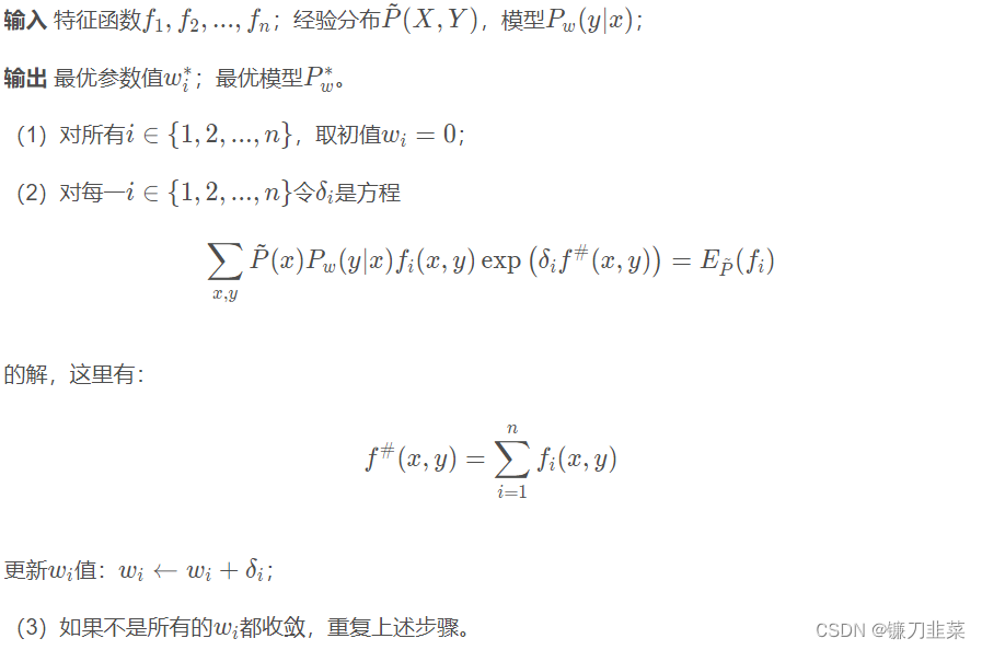
3.2 Quasi Newton method
For the maximum entropy model :
P w ( y ∣ x ) = exp ( ∑ i = 1 n w i f i ( x , y ) ) ∑ y exp ( ∑ i = 1 n w i f i ( x , y ) ) P_w(y|x)=\frac{\exp\left(\sum \limits_{i=1}^nw_if_i(x,y)\right)}{\sum \limits_{y}\exp\left(\sum \limits_{i=1}^nw_if_i(x,y)\right)} Pw(y∣x)=y∑exp(i=1∑nwifi(x,y))exp(i=1∑nwifi(x,y))
Objective function :
min w ∈ R n f ( w ) = ∑ x P ~ ( x ) log ∑ y exp ( ∑ i = 1 n w i f i ( x , y ) ) − ∑ x , y P ~ ( x , y ) ∑ i = 1 n w i f i ( x , y ) \min_{w\in\bold R^n}\ f(w)=\sum_x\tilde P(x)\log\sum_y\exp\left(\sum \limits_{i=1}^nw_if_i(x,y)\right)-\sum_{x,y}\tilde P(x,y)\sum \limits_{i=1}^nw_if_i(x,y) w∈Rnmin f(w)=x∑P~(x)logy∑exp(i=1∑nwifi(x,y))−x,y∑P~(x,y)i=1∑nwifi(x,y)
gradient :
g ( w ) = ( ∂ f ( w ) ∂ w 1 , ∂ f ( w ) ∂ w 2 , . . . , ∂ f ( w ) ∂ w n ) T g(w)=\left(\frac{\partial f(w)}{\partial w_1},\frac{\partial f(w)}{\partial w_2},...,\frac{\partial f(w)}{\partial w_n}\right)^{\rm T} g(w)=(∂w1∂f(w),∂w2∂f(w),...,∂wn∂f(w))T
among :
∂ f ( w ) ∂ w i = ∑ x , y P ~ ( x ) P w ( y ∣ x ) f i ( x , y ) − E P ~ ( f i ) , i = 1 , 2 , . . . , n \frac{\partial f(w)}{\partial w_i}=\sum_{x,y}\tilde P(x)P_w(y|x)f_i(x,y)-E_{\tilde P}(f_i),\ i=1,2,...,n ∂wi∂f(w)=x,y∑P~(x)Pw(y∣x)fi(x,y)−EP~(fi), i=1,2,...,n
Algorithm ( Quasi Newton method for maximum entropy model learning )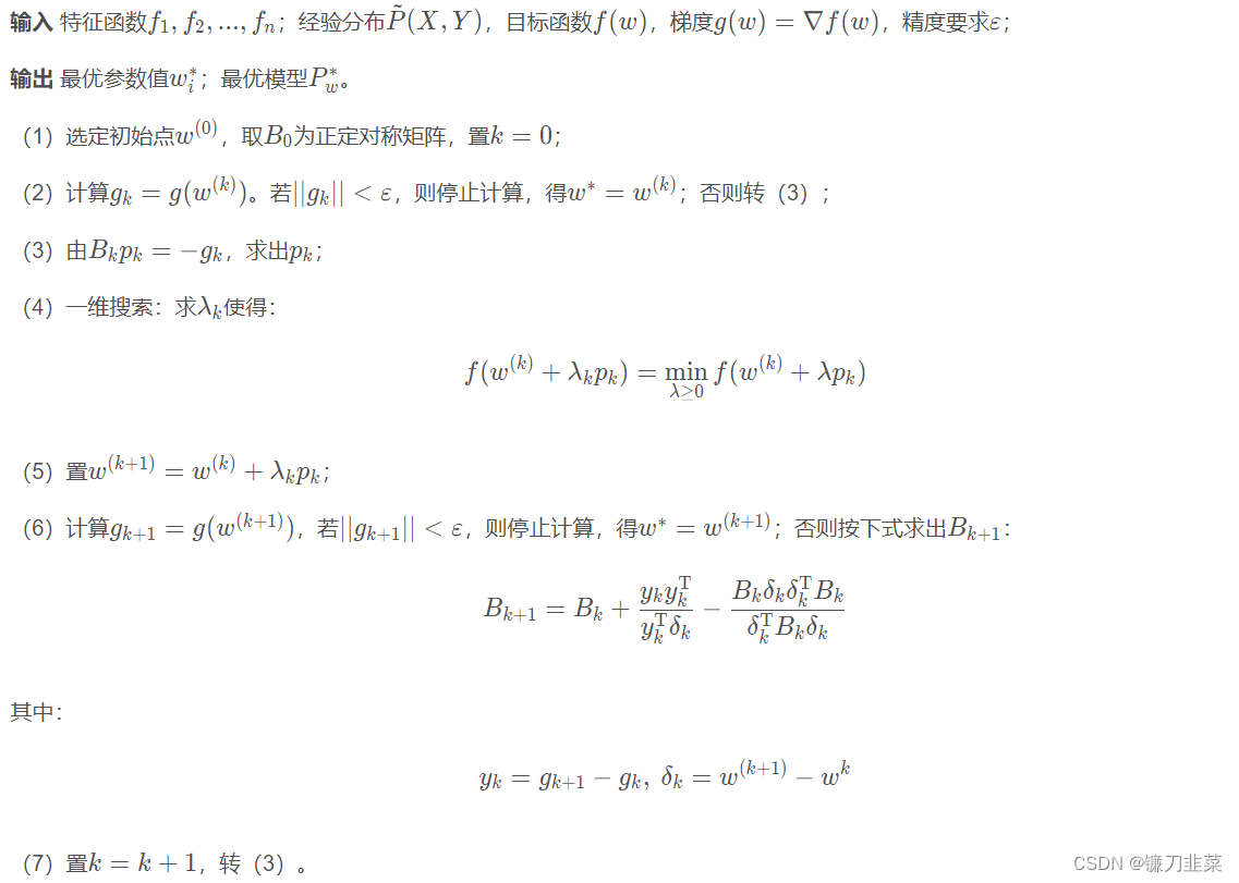
4. summary
- Logistic regression model can be used to classify two or more classes .
- Logistic regression model is a logarithmic probability model of output expressed by linear function of input .
- The principle of maximum entropy is a criterion for learning or estimating probabilistic models .
- The maximum entropy principle holds that in all possible probability models ( Distribution ) The collection of , The model with the largest entropy is the best model .
- Logistic regression model and maximum entropy model are both logarithmic linear models .
- The learning of logistic regression model and maximum entropy model generally adopts maximum likelihood estimation , Or regularized MLE .
- The learning of logistic regression model and maximum entropy model can be formalized as unconstrained optimization problem . The algorithm for solving this problem is the improved iterative scaling method 、 Gradient descent method 、 Quasi Newton method .
5. Content sources
[1] 《 Statistical learning method 》 expericnce
边栏推荐
- 浅谈估值模型 (二): PE指标II——PE Band
- Upgrade from a tool to a solution, and the new site with praise points to new value
- 【二叉树】删点成林
- Simple network configuration for equipment management
- Idea 2021 Chinese garbled code
- 【PyTorch实战】用RNN写诗
- idea 2021中文乱码
- 即刻报名|飞桨黑客马拉松第三期盛夏登场,等你挑战
- Object. Simple implementation of assign()
- 通讯协议设计与实现
猜你喜欢
In the small skin panel, use CMD to enter the MySQL command, including the MySQL error unknown variable 'secure_ file_ Priv 'solution (super detailed)
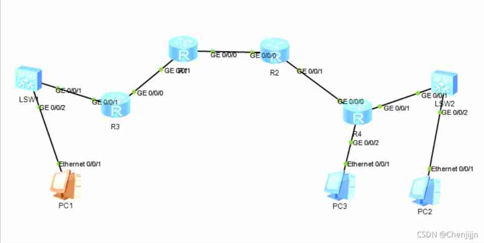
ENSP MPLS layer 3 dedicated line
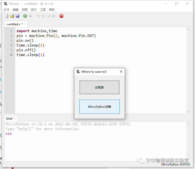
EPP+DIS学习之路(2)——Blink!闪烁!

SQL lab 21~25 summary (subsequent continuous update) (including secondary injection explanation)
![Routing strategy of multi-point republication [Huawei]](/img/5c/2e3b739ce7199f0d2a4ddd7c3856fc.jpg)
Routing strategy of multi-point republication [Huawei]
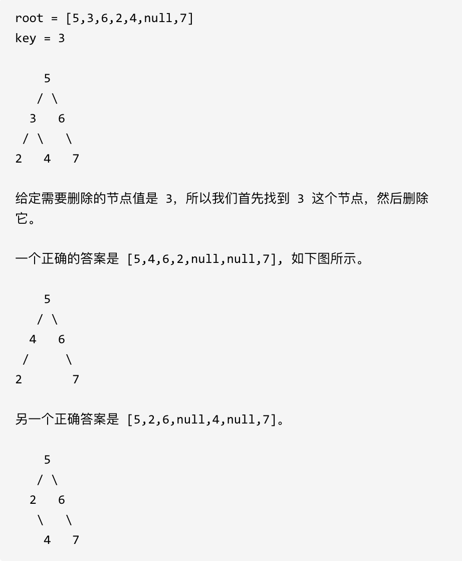
leetcode刷题:二叉树27(删除二叉搜索树中的节点)

Visual studio 2019 (localdb) \mssqllocaldb SQL Server 2014 database version is 852 and cannot be opened. This server supports version 782 and earlier
Tutorial on the principle and application of database system (011) -- relational database
Aike AI frontier promotion (7.7)
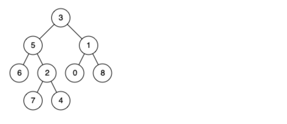
leetcode刷题:二叉树24(二叉树的最近公共祖先)
随机推荐
消息队列消息丢失和消息重复发送的处理策略
On valuation model (II): PE index II - PE band
The hoisting of the upper cylinder of the steel containment of the world's first reactor "linglong-1" reactor building was successful
leetcode刷题:二叉树27(删除二叉搜索树中的节点)
111. Network security penetration test - [privilege escalation 9] - [windows 2008 R2 kernel overflow privilege escalation]
College entrance examination composition, high-frequency mention of science and Technology
Financial data acquisition (III) when a crawler encounters a web page that needs to scroll with the mouse wheel to refresh the data (nanny level tutorial)
IPv6 experiment
What are the technical differences in source code anti disclosure
SQL lab 26~31 summary (subsequent continuous update) (including parameter pollution explanation)
wallys/Qualcomm IPQ8072A networking SBC supports dual 10GbE, WiFi 6
Aike AI frontier promotion (7.7)
NGUI-UILabel
Cenos openssh upgrade to version 8.4
跨域问题解决方案
Processing strategy of message queue message loss and repeated message sending
【统计学习方法】学习笔记——第四章:朴素贝叶斯法
利用棧來實現二進制轉化為十進制
The IDM server response shows that you do not have permission to download the solution tutorial
Is it safe to open Huatai's account in kainiu in 2022?