Recently, the weather has been extremely hot, so collect the weather data of Beijing, Shanghai, Guangzhou and Shenzhen last year, and make a visual map

Preface

The weather has been unusually hot recently , I saw that the surface temperature in some places actually reached 70°, That's ridiculous
So I want to collect weather data , Make a visualization , Recall the weather last year

development environment

• python 3.8 Run code
• pycharm 2021.2 Auxiliary knock code
• requests Third-party module

Weather data collection

1. Send a request

url = 'https://tianqi.2345.com/Pc/GetHistory?areaInfo%5BareaId%5D=54511&areaInfo%5BareaType%5D=2&date%5Byear%5D=2022&date%5Bmonth%5D=5'
response = requests.get(url)
print(response)

return <Response [200]>: The request is successful

2. get data

print(response.json())

3. Parsing data Extract the weather information

Structured data analysis ：Python Dictionary values
Unstructured data analysis ： Web page structure

json_data = response.json()
html_data = json_data['data']
select = parsel.Selector(html_data)
trs = select.css('table tr')
for tr in trs[1:]:
    #  Web page structure 
    # html Webpage  <td>asdfwaefaewfweafwaef</td> <a></a> <div></div>
    # ::text:  I need this   The text content in the tag 
    td = tr.css('td::text').getall()
    print(td)

4. Save the data

with open(' Weather data .csv', encoding='utf-8', mode='a', newline='') as f:
    csv_writer = csv.writer(f)
    csv_writer.writerow(td)

Data visualization

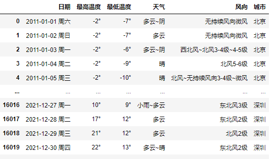
Reading data

data = pd.read_csv(' Weather data .csv')
data

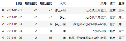
Split date / week

data[[' date ',' week ']] = data[' date '].str.split(' ',expand=True,n=1)
data

Remove redundant characters

data[[' maximum temperature ',' Minimum temperature ']] = data[[' maximum temperature ',' Minimum temperature ']].apply(lambda x: x.str.replace('°',''))
data.head()

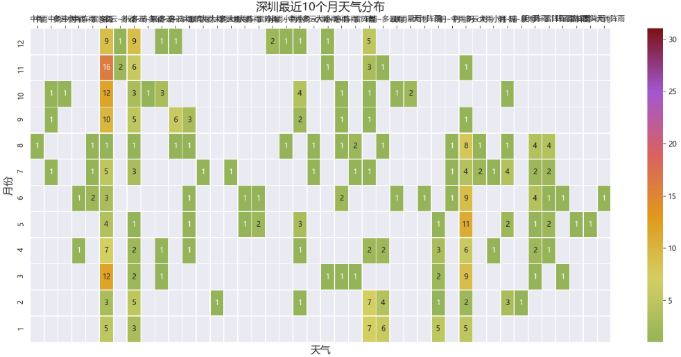
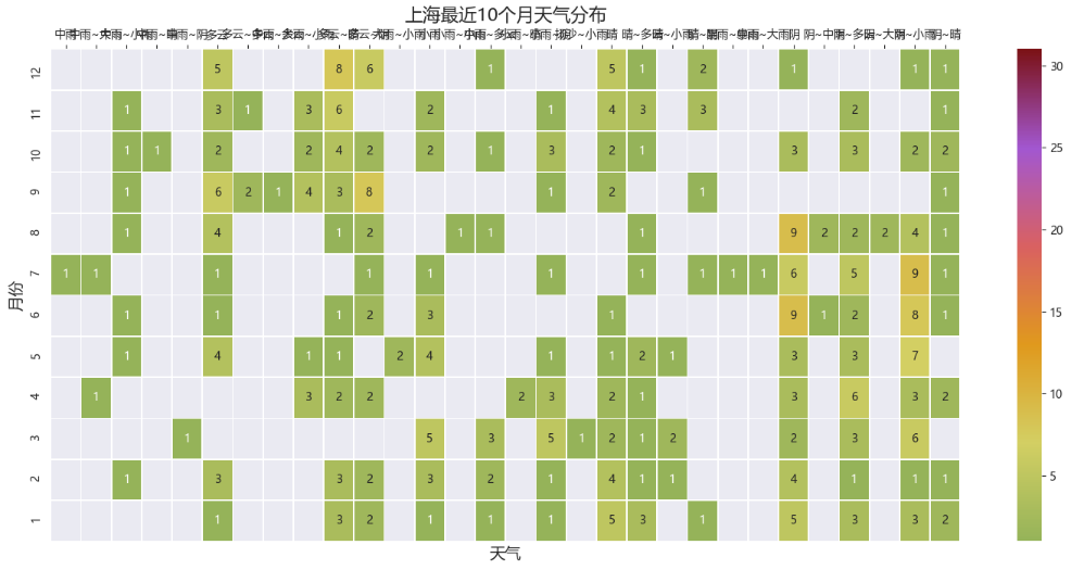
To the north, to the wide, to the deep 2021 year 10 Monthly synoptic thermodynamic map distribution

import matplotlib.pyplot as plt
import matplotlib.colors as mcolors
import seaborn as sns

# Set global default font   by   Elegant black 
plt.rcParams['font.family'] = ['Microsoft YaHei'] 
#  Set global axis label dictionary size 
plt.rcParams["axes.labelsize"] = 14  
#  Set the background 
sns.set_style("darkgrid",{
    "font.family":['Microsoft YaHei', 'SimHei']})  
#  Set canvas length and width   and  dpi
plt.figure(figsize=(18,8),dpi=100)
#  Custom color card 
cmap = mcolors.LinearSegmentedColormap.from_list("n",['#95B359','#D3CF63','#E0991D','#D96161','#A257D0','#7B1216']) 
#  Draw a heat map 

ax = sns.heatmap(data_pivot, cmap=cmap, vmax=30, 
                 annot=True, #  The values shown on the heat map 
                 linewidths=0.5,
                ) 
#  take x The axis scale is placed on the top 
ax.xaxis.set_ticks_position('top') 
plt.title(' Beijing recently 10 Monthly weather distribution ',fontsize=16) # Picture title text and font size 
plt.show()

Beijing 2021 Annual daily maximum and minimum temperature change

color0 = ['#FF76A2','#24ACE6']
color_js0 = """new echarts.graphic.LinearGradient(0, 1, 0, 0, [{offset: 0, color: '#FFC0CB'}, {offset: 1, color: '#ed1941'}], false)"""
color_js1 = """new echarts.graphic.LinearGradient(0, 1, 0, 0, [{offset: 0, color: '#FFFFFF'}, {offset: 1, color: '#009ad6'}], false)"""

tl = Timeline()
for i in range(0,len(data_bj)):
    coordy_high = list(data_bj[' maximum temperature '])[i]
    coordx = list(data_bj[' date '])[i]
    coordy_low = list(data_bj[' Minimum temperature '])[i]
    x_max = list(data_bj[' date '])[i]+datetime.timedelta(days=10)
    y_max = int(max(list(data_bj[' maximum temperature '])[0:i+1]))+3
    y_min = int(min(list(data_bj[' Minimum temperature '])[0:i+1]))-3
    title_date = list(data_bj[' date '])[i].strftime('%Y-%m-%d')
    c = (
        Line(
            init_opts=opts.InitOpts(
            theme='dark',
            # Animate 
            animation_opts=opts.AnimationOpts(animation_delay_update=800),#(animation_delay=1000, animation_easing="elasticOut"),
            # Set width 、 Height 
            width='1500px',
            height='900px', )
        )
        .add_xaxis(list(data_bj[' date '])[0:i])
        .add_yaxis(
            series_name="",
            y_axis=list(data_bj[' maximum temperature '])[0:i], is_smooth=True,is_symbol_show=False,
            linestyle_opts={
    
                   'normal': {
    
                       'width': 3,
                       'shadowColor': 'rgba(0, 0, 0, 0.5)',
                       'shadowBlur': 5,
                       'shadowOffsetY': 10,
                       'shadowOffsetX': 10,
                       'curve': 0.5,
                       'color': JsCode(color_js0)
                   }
               },
            itemstyle_opts={
    
            "normal": {
    
                "color": JsCode(
                    """new echarts.graphic.LinearGradient(0, 0, 0, 1, [{ offset: 0, color: '#ed1941' }, { offset: 1, color: '#009ad6' }], false)"""
                ),
                "barBorderRadius": [45, 45, 45, 45],
                "shadowColor": "rgb(0, 160, 221)",
            }
        },

        )
        .add_yaxis(
            series_name="",
            y_axis=list(data_bj[' Minimum temperature '])[0:i], is_smooth=True,is_symbol_show=False,
# linestyle_opts=opts.LineStyleOpts(color=color0[1],width=3),
            itemstyle_opts=opts.ItemStyleOpts(color=JsCode(color_js1)),
            linestyle_opts={
    
                   'normal': {
    
                       'width': 3,
                       'shadowColor': 'rgba(0, 0, 0, 0.5)',
                       'shadowBlur': 5,
                       'shadowOffsetY': 10,
                       'shadowOffsetX': 10,
                       'curve': 0.5,
                       'color': JsCode(color_js1)
                   }
               },
        )
        .set_global_opts(
            title_opts=opts.TitleOpts(" Beijing 2021 Annual daily maximum and minimum temperature change \n\n{}".format(title_date),pos_left=330,padding=[30,20]),
            xaxis_opts=opts.AxisOpts(type_="time",max_=x_max),#, interval=10,min_=i-5,split_number=20,axistick_opts=opts.AxisTickOpts(length=2500),axisline_opts=opts.AxisLineOpts(linestyle_opts=opts.LineStyleOpts(color="grey"))
            yaxis_opts=opts.AxisOpts(min_=y_min,max_=y_max),# Axis color ,axisline_opts=opts.AxisLineOpts(linestyle_opts=opts.LineStyleOpts(color="grey"))
        )
    )
    tl.add(c, "{}".format(list(data_bj[' date '])[i]))
    tl.add_schema(
        axis_type='time',
        play_interval=100,  #  Indicates the playback speed 
        pos_bottom="-29px",
        is_loop_play=False, #  Loop or not 
        width="780px",
        pos_left='30px',
        is_auto_play=True,  #  Auto play or not .
        is_timeline_show=False)
tl.render_notebook()

To the north, to the wide, to the deep 10 The daily maximum temperature changes in January

#  Background color 
background_color_js = (
    "new echarts.graphic.LinearGradient(0, 0, 0, 1, "
    "[{offset: 0, color: '#c86589'}, {offset: 1, color: '#06a7ff'}], false)"
)

#  Line style 
linestyle_dic = {
     'normal': {
    
                    'width': 4,  
                    'shadowColor': '#696969', 
                    'shadowBlur': 10,  
                    'shadowOffsetY': 10,  
                    'shadowOffsetX': 10,  
                    }
                }
    
timeline = Timeline(init_opts=opts.InitOpts(bg_color=JsCode(background_color_js),
                                            width='980px',height='600px'))


bj, gz, sh, sz= [], [], [], []
all_max = []
x_data = data_10[data_10[' City '] == ' Beijing '][' Japan '].tolist()
for d_time in range(len(x_data)):
    bj.append(data_10[(data_10[' Japan '] == x_data[d_time]) & (data_10[' City ']==' Beijing ')][" maximum temperature "].values.tolist()[0])
    gz.append(data_10[(data_10[' Japan '] == x_data[d_time]) & (data_10[' City ']==' Guangzhou ')][" maximum temperature "].values.tolist()[0])
    sh.append(data_10[(data_10[' Japan '] == x_data[d_time]) & (data_10[' City ']==' Shanghai ')][" maximum temperature "].values.tolist()[0])
    sz.append(data_10[(data_10[' Japan '] == x_data[d_time]) & (data_10[' City ']==' Shenzhen ')][" maximum temperature "].values.tolist()[0])
    
    line = (
        Line(init_opts=opts.InitOpts(bg_color=JsCode(background_color_js),
                                     width='980px',height='600px'))
        .add_xaxis(
            x_data,
                  )
        
        .add_yaxis(
            ' Beijing ',
            bj,
            symbol_size=5,
            is_smooth=True,
            is_hover_animation=True,
            label_opts=opts.LabelOpts(is_show=False),
        )
  
        .add_yaxis(
            ' Guangzhou ',
            gz,
            symbol_size=5,
            is_smooth=True,
            is_hover_animation=True,
            label_opts=opts.LabelOpts(is_show=False),
        )
 
        .add_yaxis(
            ' Shanghai ',
            sh,
            symbol_size=5,
            is_smooth=True,
            is_hover_animation=True,
            label_opts=opts.LabelOpts(is_show=False),
            
        )
 
        .add_yaxis(
            ' Shenzhen ',
            sz,
            symbol_size=5,
            is_smooth=True,
            is_hover_animation=True,
            label_opts=opts.LabelOpts(is_show=False),
            
        )
        
        .set_series_opts(linestyle_opts=linestyle_dic)
        .set_global_opts(
            title_opts=opts.TitleOpts(
                title=' To the north, to the wide, to the deep 10 Monthly maximum temperature change trend ',
                pos_left='center',
                pos_top='2%',
                title_textstyle_opts=opts.TextStyleOpts(color='#DC143C', font_size=20)),
            
            tooltip_opts=opts.TooltipOpts(
                trigger="axis",
                axis_pointer_type="cross",
                background_color="rgba(245, 245, 245, 0.8)",
                border_width=1,
                border_color="#ccc",
                textstyle_opts=opts.TextStyleOpts(color="#000"),
        ),
            xaxis_opts=opts.AxisOpts(
# axislabel_opts=opts.LabelOpts(font_size=14, color='red'),
# axisline_opts=opts.AxisLineOpts(is_show=True,
# linestyle_opts=opts.LineStyleOpts(width=2, color='#DB7093'))
                is_show = False
            ),
                
            
            yaxis_opts=opts.AxisOpts(
                name=' The highest temperature ',            
                is_scale=True,
# min_= int(min([gz[d_time],sh[d_time],sz[d_time],bj[d_time]])) - 10,
                max_= int(max([gz[d_time],sh[d_time],sz[d_time],bj[d_time]])) + 10,
                name_textstyle_opts=opts.TextStyleOpts(font_size=16,font_weight='bold',color='#5470c6'),
                axislabel_opts=opts.LabelOpts(font_size=13,color='#5470c6'),
                splitline_opts=opts.SplitLineOpts(is_show=True, 
                                                  linestyle_opts=opts.LineStyleOpts(type_='dashed')),
                axisline_opts=opts.AxisLineOpts(is_show=True,
                                        linestyle_opts=opts.LineStyleOpts(width=2, color='#5470c6'))
            ),
            legend_opts=opts.LegendOpts(is_show=True, pos_right='1%', pos_top='2%',
                                        legend_icon='roundRect',orient = 'vertical'),
        ))
    
    timeline.add(line, '{}'.format(x_data[d_time]))

timeline.add_schema(
    play_interval=1000,          #  Rotation speed 
    is_timeline_show=True,      #  Whether or not shown  timeline  Components 
    is_auto_play=True,          #  Auto play or not 
    pos_left="0",
    pos_right="0"
)
timeline.render_notebook()