当前位置:网站首页>Supply chain supply and demand estimation - [time series]
Supply chain supply and demand estimation - [time series]
2022-07-07 13:42:00 【Stormzudi】
Supply and demand estimation time series
Match Links :https://tianchi.aliyun.com/competition/entrance/531934/information
Coding Code :https://github.com/Stormzudi/Recommender-System-with-TF_Pytorch/tree/main/rec_examples/Works
background
The target of time series prediction is the future usage of virtual resources , Virtual resource inventory data is inventory decision 、 The time series predicts the inventory level of each inventory unit of the previous day , Inventory unit geographic topology data 、 Product topology data is the topology location information of each inventory unit , Inventory unit weight information represents the weight of each inventory unit in decision-making , A heavily weighted inventory unit , If the more effective the decision is , The contribution to the evaluation indicators will be greater ; conversely , Reducing the proportion of evaluation scores will also be greater .
This competition will focus on solving the problem in the dimension of replenishment unit ( Minimum inventory management unit ), Given the historical demand data of the past period 、 Current inventory data 、 Replenishment duration and relevant information of replenishment unit ( Product dimension and geographical latitude ), By the contestants **“ Timing prediction ”、“ Operational research optimization ” And other technologies to give the corresponding inventory management decision **, Under the condition of ensuring that the inventory probability meets the demand without supply interruption , Reduce inventory rate , Achieve the purpose of reducing inventory cost .
Data is introduced
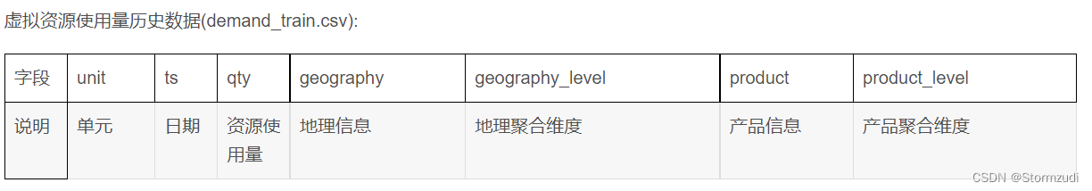
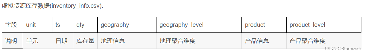
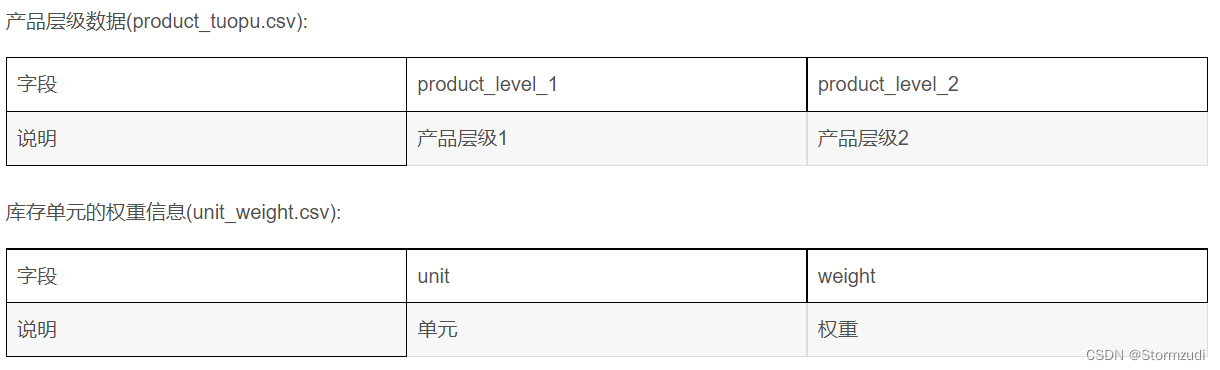
The training set contains the following : Historical data of virtual resource usage (demand_train.csv)、 Virtual resource inventory data (inventory_info.csv)、 Geographic topology data (geography_tuopu.csv)、 Product level data (product_tuopu.csv)、 Weight information of inventory unit (unit_weight.csv).

1. Feature Engineering
- 1.1 Date processing ( Make up the number of days )
- 1.2 Handle geography_level、product_level Multi level features
- 1.3 Use unit Yes qty sliding window , Add history 14 God 、7 Sky sliding window features
- 1.4 Use geo, prod Add past 14 God 、7 Sky sliding window features
1.1 Date processing
first_dt = pd.to_datetime("20180604")
last_dt = pd.to_datetime("20210301")  #  It is used to restrict the use of historical data rather than future data
start_dt = pd.to_datetime("20210301")  #  Used to define the target of the forecast test Starting time of
end_dt = pd.to_datetime("20210607")  #  Deadline for forecasting demand

demand_train_A["ts"] = demand_train_A["ts"].apply(lambda x: pd.to_datetime(x))
demand_train_A.drop(['Unnamed: 0'],axis=1,inplace=True)

demand_test_A["ts"] = demand_test_A["ts"].apply(lambda x: pd.to_datetime(x))
demand_test_A.drop(['Unnamed: 0'],axis=1,inplace=True)

dataset = pd.concat([demand_train_A, demand_test_A])
Delete incorrect sample data
#  Delete qty Samples with negative values in , The sample value of this part is incorrect , Will affect the final standardization results
dataset = dataset[~(dataset.qty < 0)]
print(np.isnan(dataset['qty']).any())
print(np.isinf(dataset['qty']).any())
dataset.info()
<class 'pandas.core.frame.DataFrame'>
Int64Index: 345316 entries, 0 to 61935
Data columns (total 7 columns):
 #   Column           Non-Null Count   Dtype
---  ------           --------------   -----
 0   unit             345316 non-null  object
 1   ts               345316 non-null  datetime64[ns]
 2   qty              345316 non-null  float64
 3   geography_level  345316 non-null  object
 4   geography        345316 non-null  object
 5   product_level    345316 non-null  object
 6   product          345316 non-null  object
dtypes: datetime64[ns](1), float64(1), object(5)
memory usage: 21.1+ MB
Check whether the days of all samples are the same
# unit count
dataset.unit.value_counts()
9b8f48bacb1a63612f3a210ccc6286cc    1100
6ed4341ad9d2902873f3d9272f5f4df1    1100
4d3ca213b639541c5ba4cf8a69b1e1ed    1100
06531cd4188630ce2497cd9983aacf5e    1100
326cb18b045e5baefa90bbc2e8d52a32    1100
                                    ...
7d9cbb373fddba4ce2cddcec96bccbeb     148
8ccf1c02bb050cb3fc4f13789cdfe235     147
e9abc1de6bd24d10ebe608959d0e5bac     141
5dbe225a546a680640eb5f7902b42cdd     141
12f892a6de3f9cf4411fb9db4fdd6691     138
Name: unit, Length: 632, dtype: int64
Every unit Make up the number of days
all_date = (dataset.ts.max()-dataset.ts.min()).days + 1
print(" Number of days for sample statistics :", all_date)  # Unit  Of   Days

#  all Unit Complete everything  all_date Days of data
cols = dataset.columns
trainalldate = pd.DataFrame()

for unit in dataset.unit.drop_duplicates():
    tmppd = pd.DataFrame(index=pd.date_range(first_dt, periods=all_date))
    tmppd['unit'] = unit
    tmppd = tmppd.reset_index()
    tmppd.columns = ['ts','unit']
    tmppd = pd.merge(left = tmppd,right = dataset[dataset.unit == unit],how = 'left',on = ['ts','unit']
        )
    #tmppd.fillna(value={'qty':-1},inplace=True)
    #tmppd.fillna(value={'qty':-1},method='bfill',inplace=True)
    trainalldate = pd.concat([trainalldate, tmppd])
Number of days for sample statistics : 1100
9b8f48bacb1a63612f3a210ccc6286cc    1100
fbb83aefc6f5d6f6bc22ae3ee757d327    1100
c667afe1760f1e611bbf1429a4d324c4    1100
159cb1b7310e185dedda75e02d75344c    1100
c33ea1a813aed8ea5c19733d0729843d    1100
                                    ...
380ad6e9d053693ab13f4da6940169ee    1100
d265d3620336f88bb6b49ac2e38c60ae    1100
e0bb0f05aa6823bddee312429820c1dc    1100
9a27f2c80de3ad06d7b57f5ec302c19e    1100
12f892a6de3f9cf4411fb9db4fdd6691    1100
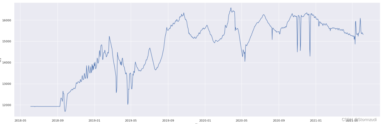
Data presentation :
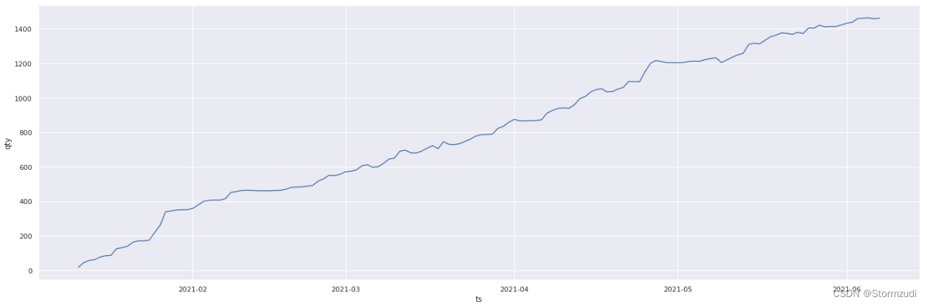
- Daily sales are complete unit: 9b8f48bacb1a63612f3a210ccc6286cc
#  Complete data
sns.set(rc={
    'figure.figsize':(25,8)})
sns.lineplot(y =trainalldate[trainalldate.unit == '9b8f48bacb1a63612f3a210ccc6286cc'].qty,
             x =trainalldate[trainalldate.unit == '9b8f48bacb1a63612f3a210ccc6286cc'].ts)
- There are days to complete unit: 7d9cbb373fddba4ce2cddcec96bccbeb
#  Incomplete data
sns.set(rc={
    'figure.figsize':(25,8)})
sns.lineplot(y =trainalldate[trainalldate.unit == '7d9cbb373fddba4ce2cddcec96bccbeb'].qty,
             x =trainalldate[trainalldate.unit == '7d9cbb373fddba4ce2cddcec96bccbeb'].ts)
add to year, month, day Date characteristics
trainalldate['year'] = trainalldate['ts'].dt.year
trainalldate['month'] = trainalldate['ts'].dt.month
trainalldate['day'] = trainalldate['ts'].dt.day
trainalldate['week'] = trainalldate['ts'].dt.weekday
trainalldate.info()
<class 'pandas.core.frame.DataFrame'>
Int64Index: 695200 entries, 0 to 1099
Data columns (total 11 columns):
 #   Column           Non-Null Count   Dtype
---  ------           --------------   -----
 0   ts               695200 non-null  datetime64[ns]
 1   unit             695200 non-null  object
 2   qty              345316 non-null  float64
 3   geography_level  345316 non-null  object
 4   geography        345316 non-null  object
 5   product_level    345316 non-null  object
 6   product          345316 non-null  object
 7   year             695200 non-null  int64
 8   month            695200 non-null  int64
 9   day              695200 non-null  int64
 10  week             695200 non-null  int64
dtypes: datetime64[ns](1), float64(1), int64(4), object(5)
memory usage: 63.6+ MB
1.2 Handle geography_level、product_level Multi level features
trainalldate = trainalldate.drop(['geography_level','product_level'],axis = 1)
trainalldate = pd.merge(trainalldate, geo_topo, how='left', left_on = 'geography', right_on = 'geography_level_3')
trainalldate = pd.merge(trainalldate, product_topo, how='left', left_on = 'product', right_on = 'product_level_2')
trainalldate = trainalldate.drop(['geography','product'],axis = 1)
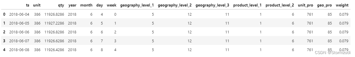
trainalldate.head()
Conduct label encoder, Implement character type -> Numerical type
# labelEncoder
encoder = ['geography_level_1','geography_level_2','geography_level_3','product_level_1','product_level_2']
# add feature
# unit_all = ['unit_geo', 'unit_pro', 'geo_pro']
unit_all = [ 'unit_pro', 'geo_pro']

# trainalldate["unit_geo"] = trainalldate.apply(lambda x: f"{x['unit']}_{x['geography_level_3']}", axis=1)
trainalldate["unit_pro"] = trainalldate.apply(lambda x: f"{
      x['unit']}_{
      x['product_level_2']}", axis=1)
trainalldate["geo_pro"] = trainalldate.apply(lambda x: f"{
      x['geography_level_3']}_{
      x['product_level_2']}", axis=1)

lbl = LabelEncoder()
for feat in encoder+unit_all:
    lbl.fit(trainalldate[feat])
    trainalldate[feat] = lbl.transform(trainalldate[feat])
Add Training weight characteristics : weight
# add the weight of each units
trainalldate = pd.merge(trainalldate, weight_A, left_on = 'unit', right_on = 'unit')
trainalldate = trainalldate.drop(['Unnamed: 0'],axis = 1)
For the prediction target qty Conduct label encoder code
# unit to unit_id
enc_unit = lbl.fit(trainalldate['unit'])
trainalldate['unit'] = enc_unit.transform(trainalldate['unit'])
trainalldate.head()

# unit id ->  Anti coding
# enc_unit.inverse_transform(trainalldate['unit'])
Storage .pkl file
# save to pkl
# trainalldate.to_csv('../output/trainalldate.csv', index=False)
import pickle

with open("../output/trainalldate.pkl", 'wb') as fo:
    pickle.dump(trainalldate, fo)
1.3 Use unit Yes qty sliding window , Add history 14 God 、7 Sky sliding window features
ref: https://zhuanlan.zhihu.com/p/101284491
with open("../output/trainalldate.pkl", 'rb') as fo:     #  Read pkl File data
    trainalldate = pickle.load(fo, encoding='bytes')

trainalldate["ts"] = trainalldate["ts"].apply(lambda x: pd.to_datetime(x))  #  Convert to time format
print(trainalldate.shape)
trainalldate.head()
- history 14 God 7 Sliding window
- History No k Day specific value ( The third day of history , The second day of history , yesterday )
def qtyGetKvalue(data, k):
    ''' k: the last k-ist value of data '''
    data = data.sort_values(
        by=['ts'], ascending=True).reset_index(drop=True)
    data = data.iloc[len(data) - k, -1] if len(data) >= k else np.NaN
    return data

def qtyNewFeature(df, ts = np.nan):
    newdataset = pd.DataFrame()

    timeline = pd.date_range(df.ts.min(), df.ts.max())
    for t in timeline:

        # today
        ts = df[df.ts == t]

        # last 14 day information ...
        rdd = df[(df.ts >= t - datetime.timedelta(14)) & (df.ts < t)]

        last14max_dict = rdd.groupby('unit')['qty'].max().to_dict()
        last14min_dict = rdd.groupby('unit')['qty'].min().to_dict()
        last14std_dict = rdd.groupby('unit')['qty'].std().to_dict()
        last14mean_dict = rdd.groupby('unit')['qty'].mean().to_dict()
        last14median_dict = rdd.groupby('unit')['qty'].median().to_dict()
        last14sum_dict = rdd.groupby('unit')['qty'].sum().to_dict()

        ts['last14max'] = ts['unit'].map(last14max_dict)
        ts['last14min'] = ts['unit'].map(last14min_dict)
        ts['last14std'] = ts['unit'].map(last14std_dict)
        ts['last14mean'] = ts['unit'].map(last14mean_dict)
        ts['last14median'] = ts['unit'].map(last14median_dict)
        ts['last14sum'] = ts['unit'].map(last14sum_dict)


        # last 7 day information ..
        rdd = df[(df.ts >= t - datetime.timedelta(7)) & (df.ts < t)]

        last7max_dict = rdd.groupby('unit')['qty'].max().to_dict()
        last7min_dict = rdd.groupby('unit')['qty'].min().to_dict()
        last7std_dict = rdd.groupby('unit')['qty'].std().to_dict()
        last7mean_dict = rdd.groupby('unit')['qty'].mean().to_dict()
        last7median_dict = rdd.groupby('unit')['qty'].median().to_dict()
        last7sum_dict = rdd.groupby('unit')['qty'].sum().to_dict()

        ts['last7max'] = ts['unit'].map(last7max_dict)
        ts['last7min'] = ts['unit'].map(last7min_dict)
        ts['last7std'] = ts['unit'].map(last7std_dict)
        ts['last7mean'] = ts['unit'].map(last7mean_dict)
        ts['last7median'] = ts['unit'].map(last7median_dict)
        ts['last7sum'] = ts['unit'].map(last7sum_dict)


        # last 3 day information ...
        rdd = df[(df.ts >= t - datetime.timedelta(3)) & (df.ts < t)]

        last3max_dict = rdd.groupby('unit')['qty'].max().to_dict()
        last3min_dict = rdd.groupby('unit')['qty'].min().to_dict()
        last3std_dict = rdd.groupby('unit')['qty'].std().to_dict()
        last3mean_dict = rdd.groupby('unit')['qty'].mean().to_dict()
        last3median_dict = rdd.groupby('unit')['qty'].median().to_dict()
        last3sum_dict = rdd.groupby('unit')['qty'].sum().to_dict()
        last3value_dict = rdd.groupby('unit')['ts', 'qty'].apply(qtyGetKvalue, k=3).to_dict()

        ts['last3max'] = ts['unit'].map(last3max_dict)
        ts['last3min'] = ts['unit'].map(last3min_dict)
        ts['last3std'] = ts['unit'].map(last3std_dict)
        ts['last3mean'] = ts['unit'].map(last3mean_dict)
        ts['last3median'] = ts['unit'].map(last3median_dict)
        ts['last3sum'] = ts['unit'].map(last3sum_dict)
        ts['last3value'] = ts['unit'].map(last3value_dict)


        # last 1、2 day information ..
        rdd = df[(df.ts >= t - datetime.timedelta(1)) & (df.ts < t)]
        last1value_dict = rdd.groupby('unit')['qty'].sum().to_dict()
        ts['last1value'] = ts['unit'].map(last1value_dict)

        rdd = df[(df.ts >= t - datetime.timedelta(2)) & (df.ts < t)]
        last2mean_dict = rdd.groupby('unit')['qty'].mean().to_dict()
        last2sum_dict = rdd.groupby('unit')['qty'].sum().to_dict()
        last2value_dict = rdd.groupby('unit')['ts', 'qty'].apply(qtyGetKvalue, k=2).to_dict()

        ts['last2mean'] = ts['unit'].map(last2mean_dict)
        ts['last2sum'] = ts['unit'].map(last2sum_dict)
        ts['last2value'] = ts['unit'].map(last2value_dict)

        newdataset = pd.concat([newdataset, ts])
        if t.month == 1 and t.day == 1:
            print(t)
    return newdataset
run…
traindataset = qtyNewFeature(trainalldate)
<class 'pandas.core.frame.DataFrame'>
Int64Index: 695200 entries, 0 to 695199
Data columns (total 38 columns):
 #   Column             Non-Null Count   Dtype
---  ------             --------------   -----
 0   ts                 695200 non-null  datetime64[ns]
 1   unit               695200 non-null  int64
 2   qty                345316 non-null  float64
 3   year               695200 non-null  int64
 4   month              695200 non-null  int64
 5   day                695200 non-null  int64
 6   week               695200 non-null  int64
 7   geography_level_1  695200 non-null  int64
 8   geography_level_2  695200 non-null  int64
 9   geography_level_3  695200 non-null  int64
 10  product_level_1    695200 non-null  int64
 11  product_level_2    695200 non-null  int64
 12  unit_pro           695200 non-null  int64
 13  geo_pro            695200 non-null  int64
 14  weight             695200 non-null  float64
 15  last14max          344717 non-null  float64
 16  last14min          344717 non-null  float64
 17  last14std          344085 non-null  float64
 18  last14mean         344717 non-null  float64
 19  last14median       344717 non-null  float64
 20  last14sum          694568 non-null  float64
 21  last7max           344712 non-null  float64
 22  last7min           344712 non-null  float64
 23  last7std           344068 non-null  float64
 24  last7mean          344712 non-null  float64
 25  last7median        344712 non-null  float64
 26  last7sum           694568 non-null  float64
 27  last3max           344695 non-null  float64
 28  last3min           344695 non-null  float64
 29  last3std           344051 non-null  float64
 30  last3mean          344695 non-null  float64
 31  last3median        344695 non-null  float64
 32  last3sum           694568 non-null  float64
 33  last3value         344684 non-null  object
 34  last1value         694568 non-null  float64
 35  last2mean          344690 non-null  float64
 36  last2sum           694568 non-null  float64
 37  last2value         344684 non-null  object
dtypes: datetime64[ns](1), float64(23), int64(12), object(2)
memory usage: 206.9+ MB
1.4 Use geo, prod Add past 14 God 、7 Sky sliding window features
def geoproNewFeature(df):
    newdataset = pd.DataFrame()

    timeline = pd.date_range(df.ts.min(), df.ts.max())
    for t in timeline:
        ts = df[df.ts == t]
        rdd = df[(df.ts >= t - datetime.timedelta(14)) & (df.ts < t)]

        # grouby for calculate mean&median
        geo1mean14_dict = rdd.groupby('geography_level_1')['qty'].mean().to_dict()
        geo2mean14_dict = rdd.groupby('geography_level_2')['qty'].mean().to_dict()
        geo3mean14_dict = rdd.groupby('geography_level_3')['qty'].mean().to_dict()
        pro1mean14_dict = rdd.groupby('product_level_1')['qty'].mean().to_dict()
        pro2mean14_dict = rdd.groupby('product_level_2')['qty'].mean().to_dict()
        geo1median14_dict = rdd.groupby('geography_level_1')['qty'].median().to_dict()
        geo2median14_dict = rdd.groupby('geography_level_2')['qty'].median().to_dict()
        geo3median14_dict = rdd.groupby('geography_level_3')['qty'].median().to_dict()
        pro1median14_dict = rdd.groupby('product_level_1')['qty'].median().to_dict()
        pro2median14_dict = rdd.groupby('product_level_2')['qty'].median().to_dict()

        # map to df
        ts['geo1mean14'] = ts['geography_level_1'].map(geo1mean14_dict)
        ts['geo2mean14'] = ts['geography_level_2'].map(geo2mean14_dict)
        ts['geo3mean14'] = ts['geography_level_3'].map(geo3mean14_dict)
        ts['pro1mean14'] = ts['product_level_1'].map(pro1mean14_dict)
        ts['pro2mean14'] = ts['product_level_2'].map(pro2mean14_dict)

        ts['geo1median14'] = ts['geography_level_1'].map(geo1median14_dict)
        ts['geo2median14'] = ts['geography_level_2'].map(geo2median14_dict)
        ts['geo3median14'] = ts['geography_level_3'].map(geo3median14_dict)
        ts['pro1median14'] = ts['product_level_1'].map(pro1median14_dict)
        ts['pro2median14'] = ts['product_level_2'].map(pro2median14_dict)
add to geo and prod Under the Sliding window features :
traindatasetall = geoproNewFeature(traindataset)
traindatasetall.info()
<class 'pandas.core.frame.DataFrame'>
Int64Index: 695200 entries, 0 to 695199
Data columns (total 48 columns):
 #   Column             Non-Null Count   Dtype
---  ------             --------------   -----
 0   ts                 695200 non-null  datetime64[ns]
 1   unit               695200 non-null  int64
 2   qty                345316 non-null  float64
 3   year               695200 non-null  int64
 4   month              695200 non-null  int64
 5   day                695200 non-null  int64
 6   week               695200 non-null  int64
 7   geography_level_1  695200 non-null  int64
 8   geography_level_2  695200 non-null  int64
 9   geography_level_3  695200 non-null  int64
 10  product_level_1    695200 non-null  int64
 11  product_level_2    695200 non-null  int64
 12  unit_pro           695200 non-null  int64
 13  geo_pro            695200 non-null  int64
 14  weight             695200 non-null  float64
 15  last14max          344717 non-null  float64
 16  last14min          344717 non-null  float64
 17  last14std          344085 non-null  float64
 18  last14mean         344717 non-null  float64
 19  last14median       344717 non-null  float64
 20  last14sum          694568 non-null  float64
 21  last7max           344712 non-null  float64
 22  last7min           344712 non-null  float64
 23  last7std           344068 non-null  float64
 24  last7mean          344712 non-null  float64
 25  last7median        344712 non-null  float64
 26  last7sum           694568 non-null  float64
 27  last3max           344695 non-null  float64
 28  last3min           344695 non-null  float64
 29  last3std           344051 non-null  float64
 30  last3mean          344695 non-null  float64
 31  last3median        344695 non-null  float64
 32  last3sum           694568 non-null  float64
 33  last3value         344684 non-null  object
 34  last1value         694568 non-null  float64
 35  last2mean          344690 non-null  float64
 36  last2sum           694568 non-null  float64
 37  last2value         344684 non-null  object
 38  geo1mean14         345294 non-null  float64
 39  geo2mean14         345267 non-null  float64
 40  geo3mean14         345198 non-null  float64
 41  pro1mean14         344949 non-null  float64
 42  pro2mean14         344946 non-null  float64
 43  geo1median14       345294 non-null  float64
 44  geo2median14       345267 non-null  float64
 45  geo3median14       345198 non-null  float64
 46  pro1median14       344949 non-null  float64
 47  pro2median14       344946 non-null  float64
dtypes: datetime64[ns](1), float64(33), int64(12), object(2)
memory usage: 259.9+ MB
2. Data analysis
- 2.1 Date and inventory sales qty The relationship between
- 2.2 weight Analysis between characteristics and other indicators
- 2.3 geography and product And inventory sales qty The relationship between
2.1 Date and inventory sales qty The relationship between
- 1. Which month has the best inventory sales , As the date changes , What is the change trend of average inventory sales ?
- 2. Which day of the month has the best inventory sales ?
#  Statistics 2020-1-1  to  2021-1-1  Sales between days
l = pd.to_datetime("20200101")
r = pd.to_datetime("20210101")
rdd = trainalldate[(trainalldate.ts >= l) & (trainalldate.ts < r)]
rdd.groupby('month')['qty'].mean().plot.line()
rdd.groupby('month')['qty'].mean()
month
1     7192.430061
2     7314.206949
3     7604.787311
4     7816.873783
5     7654.873306
6     7414.775432
7     7338.711291
8     7143.824906
9     6443.558908
10    6322.372180
11    6342.427577
12    6338.860666
Name: qty, dtype: float64
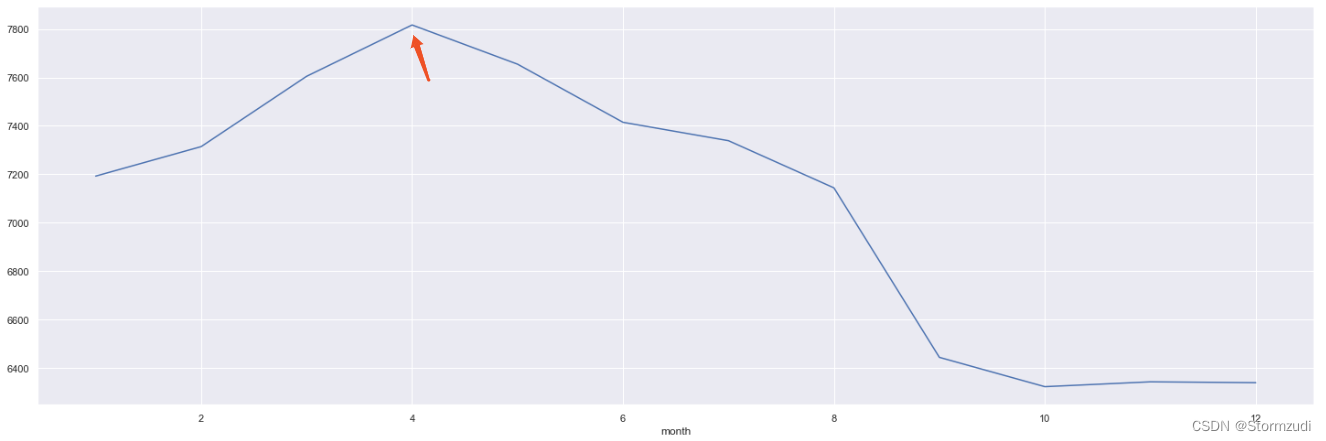
In a year 4 Each month unit Of Best sales .
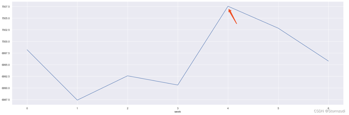
rdd.groupby('week')['qty'].mean().plot.line()
rdd.groupby('week')['qty'].mean()
week
0    6998.214075
1    6987.379158
2    6992.602257
3    6990.622916
4    7007.556214
5    7002.836863
6    6995.769412
Name: qty, dtype: float64
rdd.groupby('day')['qty'].mean().plot.line()
rdd.groupby('day')['qty'].mean()
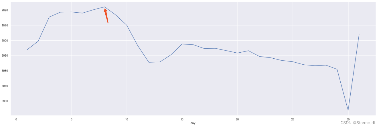
# the high day is 8
# count the 8 of all year
daysYear = pd.Series(pd.date_range(start=l, end=r))
weeks = list(map(lambda x:x.day_name(), filter(lambda x:x.day == 8, daysYear)))
print(list(filter(lambda x:x.day == 8, daysYear)))
print(weeks)
import collections
a = collections.Counter(weeks)
plt.bar(*zip(*a.items()))
plt.show()
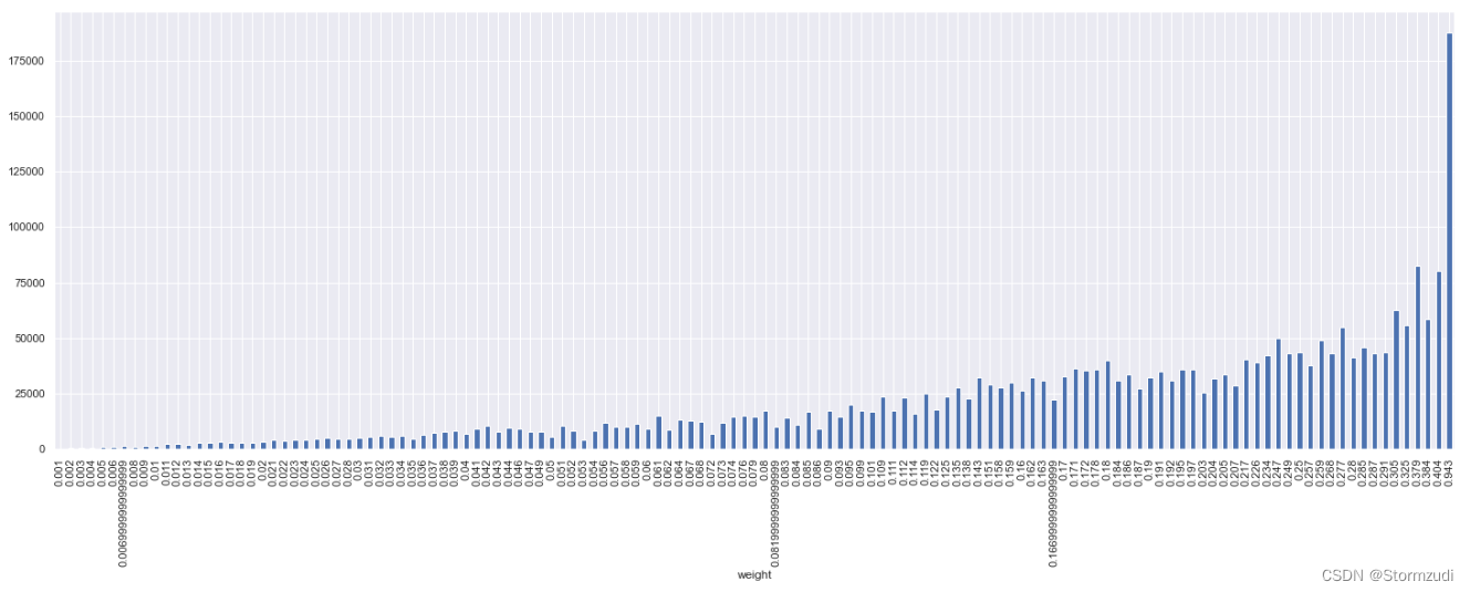
2.2 weight Characteristics analysis
# weight num and unit
trainalldate.groupby('weight')['unit'].count()
weight
0.001    139700
0.002     62700
0.003     52800
0.004     31900
0.005     31900
          ...
0.325      1100
0.379      1100
0.384      1100
0.404      1100
0.943      1100
Name: unit, Length: 131, dtype: int64
All in all 131 Different species weight, Most of them weight == 0.001
#  Statistical difference weight Next ,qty Average inventory usage
trainalldate.groupby('weight')['qty'].mean().plot.bar()
2.3 geography and product And inventory sales qty The relationship between
3. model training
- 1 Xgboost
- 2.LightGBM
- 3.autox
- 4.JDCross
- ref
https://github.com/PENGZhaoqing/TimeSeriesPrediction
https://github.com/gabrielpreda/Kaggle/blob/master/SantanderCustomerTransactionPrediction/starter-code-saving-and-loading-lgb-xgb-cb.py
3.1 xgboost
# load traindataset
with open("../output/traindataset.pkl", 'rb') as fo:     #  Read pkl File data
    traindataset = pickle.load(fo, encoding='bytes')

traindataset["ts"] = traindataset["ts"].apply(lambda x: pd.to_datetime(x))
print(traindataset.shape)
traindataset.head()
# features
sparse_features = ['unit', 'year', 'month', 'day', 'week', 'geography_level_1', 'geography_level_2', 'geography_level_3',
                   'product_level_1', 'product_level_2', 'unit_pro', 'geo_pro']
dense_features = ['weight',
       'last14max', 'last14min', 'last14std', 'last14mean', 'last14median',
       'last14sum', 'last7max', 'last7min', 'last7std', 'last7mean',
       'last7median', 'last7sum', 'last3max', 'last3min', 'last3std',
       'last3mean', 'last3median', 'last3sum', 'last3value', 'last1value', 'last2mean',
       'last2sum', 'last2value', 'geo1mean14', 'geo2mean14', 'geo3mean14', 'pro1mean14',
       'pro2mean14', 'geo1median14', 'geo2median14', 'geo3median14',
       'pro1median14', 'pro2median14']

target = ['qty']
# traindataset[:100].loc[~traindataset[:100]['geo1mean14'].isnull()]
# traindataset[np.isnan(traindataset['qty'].values)]
# traindataset['qty'][np.isinf(traindataset['qty'])] = 0.0

#  Replace null , And select greater than 0 The data of
traindataset = traindataset.dropna(subset=["qty"])
traindataset = traindataset[traindataset["qty"] >= 0]
traindataset.shape
(345316, 48)
Judge whether it exists Null and inf outliers .
print(np.isnan(traindataset['qty']).any())
print(np.isinf(traindataset['qty']).any())
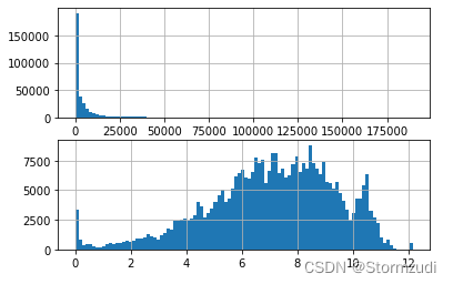
qty The original value is too large , Conduct log conversion .
# qty  To convert
plt.figure(figsize=(18, 10))
fig, axes = plt.subplots(nrows=2, ncols=1)
traindataset['qty'].hist(bins=100, ax=axes[0])
traindataset['qty'] = np.log(traindataset['qty'] + 1)  #
traindataset['qty'].hist(bins=100, ax=axes[1])
plt.show()
## 3.1 xgboost
traindataset = traindataset.dropna(axis=0, how='any')
train = traindataset[traindataset.ts <= pd.to_datetime("20210301")]
test = traindataset[traindataset.ts > pd.to_datetime("20210301")]

X_train, X_test, y_train, y_test = train[sparse_features + dense_features], test[sparse_features + dense_features], train[target], test[target]
print('The shape of X_train:{}'.format(X_train.shape))
print('The shape of X_test:{}'.format(X_test.shape))
The shape of X_train:(274740, 46)
The shape of X_test:(68685, 46)
params = {

    'learning_rate': 0.25,
    'n_estimators': 30,
    'subsample': 0.8,
    'colsample_bytree': 0.6,
    'max_depth': 12,
    'min_child_weight': 1,
    'reg_alpha': 0,
    'gamma': 0
}

# dtrain = xgb.DMatrix(X, label=y, feature_names=x)

bst = xgb.XGBRegressor(learning_rate=params['learning_rate'], n_estimators=params['n_estimators'],
                             booster='gbtree', objective='reg:linear', n_jobs=-1, subsample=params['subsample'],
                             colsample_bytree=params['colsample_bytree'], random_state=0,
                             max_depth=params['max_depth'], gamma=params['gamma'],
                             min_child_weight=params['min_child_weight'], reg_alpha=params['reg_alpha'])
bst.fit(X_train.values, y_train.values)
[15:50:29] WARNING: ../src/objective/regression_obj.cu:203: reg:linear is now deprecated in favor of reg:squarederror.[134]:
XGBRegressor(base_score=0.5, booster='gbtree', callbacks=None,
             colsample_bylevel=1, colsample_bynode=1, colsample_bytree=0.6,
             early_stopping_rounds=None, enable_categorical=False,
             eval_metric=None, gamma=0, gpu_id=-1, grow_policy='depthwise',
             importance_type=None, interaction_constraints='',
             learning_rate=0.25, max_bin=256, max_cat_to_onehot=4,
             max_delta_step=0, max_depth=12, max_leaves=0, min_child_weight=1,
             missing=nan, monotone_constraints='()', n_estimators=30, n_jobs=-1,
             num_parallel_tree=1, objective='reg:linear', predictor='auto',
             random_state=0, reg_alpha=0, ...)
View the prediction effect
pre = bst.predict(X_test.values)

# def mape(y_true, y_pred):
# return np.mean(np.abs((y_pred - y_true) / y_true)) * 100

# mape = mape(np.expm1(y_test.reshape(-1)), np.expm1(pre))
# print("MAPE is: {}".format(mape))

from sklearn.metrics import mean_absolute_error, mean_squared_error
mae_norm = mean_absolute_error(y_test.values, pre)  #  Normalized value
mae = mean_absolute_error(np.expm1(y_test.values), np.expm1(pre))


rmse = np.sqrt(mean_squared_error(np.expm1(y_test.values), np.expm1(pre)))

print("mae:",mae_norm)
print("mae:",mae)
print("rmse:",rmse)
mae: 0.0169853220505046
mae: 56.53049660927482
rmse: 232.05474656993192
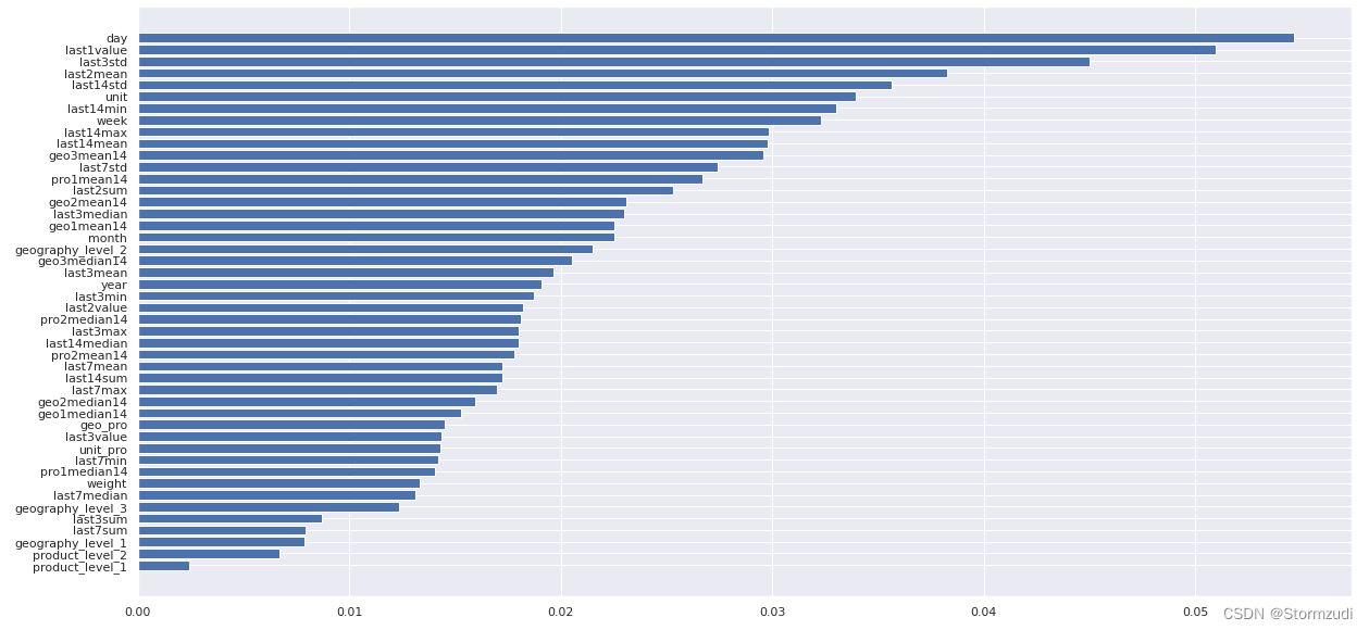
The importance diagram of tree model output eigenvalues
def get_xgb_feat_importances(clf, train_features):

    if isinstance(clf, xgb.XGBModel):
        # clf has been created by calling
        # xgb.XGBClassifier.fit() or xgb.XGBRegressor().fit()
        fscore = clf.get_booster().get_fscore()
    else:
        # clf has been created by calling xgb.train.
        # Thus, clf is an instance of xgb.Booster.
        fscore = clf.get_fscore()

    feat_importances = []

    for feat, value in zip(fscore.keys(), train_features):
        feat_importances.append({
    'Feature': value, 'Importance': fscore[feat]})

    # for ft, score in fscore.items():
    # feat_importances.append({'Feature': ft, 'Importance': score})
    feat_importances = pd.DataFrame(feat_importances)
    feat_importances = feat_importances.sort_values(
        by='Importance', ascending=False).reset_index(drop=True)
    # Divide the importances by the sum of all importances
    # to get relative importances. By using relative importances
    # the sum of all importances will equal to 1, i.e.,
    # np.sum(feat_importances['importance']) == 1
    feat_importances['Importance'] /= feat_importances['Importance'].sum()
    # Print the most important features and their importances
    return dict(zip(fscore.keys(), train_features)), feat_importances


f, res = get_xgb_feat_importances(bst, sparse_features + dense_features)

plt.figure(figsize=(20, 10))
plt.barh(range(len(res)), res['Importance'][::-1], tick_label=res['Feature'][::-1])
plt.show()
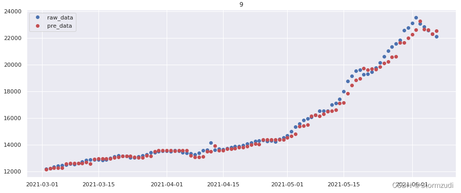
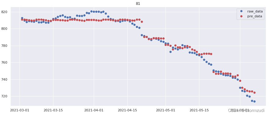
View the prediction effect
# plot the model result

data = X_test.copy()
data['qty'] = np.expm1(y_test)
data['pre_qty'] = np.expm1(pre)

def date_trend(data):
    val = data.sort_values(
        by=['year', 'month', 'day'], ascending=True).reset_index(drop=True)

    val["date"] = val.apply(lambda x: f"{
      int(x['year'])}-{
      int(x['month'])}-{
      int(x['day'])}", axis=1)
    val["date"] = val["date"].apply(lambda x: pd.to_datetime(x))

    if val.unit.values[0] in [497, 81, 9, 285, 554, 315]:
        plt.figure(figsize=(15, 6))
        l1 = plt.plot(val.date, val['qty'], 'o', label='raw_data')
        l2 = plt.plot(val.date, val['pre_qty'], 'ro', label="pre_data")
        plt.legend()
        # plt.plot(val.date, val['qty'], 'o', val.date, val['pre_qty'], 'ro')
        plt.title(str(val.unit.values[0]))
        plt.show()


data.groupby('unit').apply(date_trend)
3.2 Lightgbm
import lightgbm as lgb
from lightgbm import plot_importance


#  Build a training set
dtrain = lgb.Dataset(X_train,y_train)
dtest = lgb.Dataset(X_test,y_test)

params = {

    'booster': 'gbtree',
    'objective': 'regression',
    'num_leaves': 31,
    'subsample': 0.8,
    'bagging_freq': 1,
    'feature_fraction ': 0.8,
    'slient': 1,
    'learning_rate ': 0.1,
    'seed': 0
}

num_rounds = 500

# xgboost model training
lgbmodel = lgb.train(params,dtrain, num_rounds, valid_sets=[dtrain, dtest],
                  verbose_eval=100, early_stopping_rounds=100)

#  Predict the test set
pre_lgb = lgbmodel.predict(X_test)
Evaluate the effect of the model
# def mape(y_true, y_pred):
# return np.mean(np.abs((y_pred - y_true) / y_true)) * 100

# mape = mape(np.expm1(y_test.reshape(-1)), np.expm1(pre))
# print("MAPE is: {}".format(mape))

from sklearn.metrics import mean_absolute_error, mean_squared_error
mae_norm = mean_absolute_error(y_test.values, pre_lgb)  #  Normalized value
mae = mean_absolute_error(np.expm1(y_test.values), np.expm1(pre_lgb))


rmse = np.sqrt(mean_squared_error(np.expm1(y_test.values), np.expm1(pre_lgb)))

print("mae:",mae_norm)
print("mae:",mae)
print("rmse:",rmse)
mae: 0.018923955297323495
mae: 81.15812502488455
rmse: 307.6095513832293
边栏推荐
- mysql 局域网内访问不到的问题
- JS determines whether an object is empty
- How to make join run faster?
- .net core 关于redis的pipeline以及事务
- [dark horse morning post] Huawei refutes rumors about "military master" Chen Chunhua; Hengchi 5 has a pre-sale price of 179000 yuan; Jay Chou's new album MV has played more than 100 million in 3 hours
- Solve the cache breakdown problem
- Mongodb slice summary
- What parameters need to be reconfigured to replace the new radar of ROS robot
- 【堡垒机】云堡垒机和普通堡垒机的区别是什么?
- Clion mingw64 Chinese garbled code
猜你喜欢

作战图鉴:12大场景详述容器安全建设要求

2022-7-6 使用SIGURG来接受外带数据,不知道为什么打印不出来

PAcP learning note 1: programming with pcap

Final review notes of single chip microcomputer principle

Custom thread pool rejection policy

Getting started with MySQL
![[learning notes] agc010](/img/2c/37f2537a4dadd84adacf3da5f1327a.png)
[learning notes] agc010

1. Deep copy 2. Call apply bind 3. For of in differences

Vscade editor esp32 header file wavy line does not jump completely solved
1、深拷贝 2、call apply bind 3、for of for in 区别
随机推荐
PHP - laravel cache
Data refresh of recyclerview
Mongodb meets spark (for integration)
toRaw和markRaw
华为镜像地址
提升树莓派性能的方法
2022-7-6 Leetcode 977.有序数组的平方
MongoDB优化的几点原则
【日常训练】648. 单词替换
SSRF漏洞file伪协议之[网鼎杯 2018]Fakebook1
室內ROS機器人導航調試記錄(膨脹半徑的選取經驗)
最佳实践 | 用腾讯云AI意愿核身为电话合规保驾护航
[daily training -- Tencent select 50] 231 Power of 2
Co create a collaborative ecosystem of software and hardware: the "Joint submission" of graphcore IPU and Baidu PaddlePaddle appeared in mlperf
RealBasicVSR测试图片、视频
PAcP learning note 3: pcap method description
Solve the cache breakdown problem
单片机学习笔记之点亮led 灯
Thread pool reject policy best practices
postgresql array类型,每一项拼接