当前位置:网站首页>Application of machine learning in housing price prediction
Application of machine learning in housing price prediction
2022-07-04 23:11:00 【Wu_ Candy】
Preface
Python It has natural advantages in machine learning , So let's also get involved in the technology of machine learning today , Here are some notes from the learning process , There are a lot of notes in it , Used to understand why this is done .
See the article on resource sharing for the data involved -- machine learning - Data sets ( Forecast house prices )
The code implementation is as follows :
Numpy & Pandas & Matplotlib & Ipython
#NumPy(Numerical Python)  yes  Python  An extended library of language , Support a large number of dimension arrays and matrix operations , In addition, it also provides a large number of mathematical function libraries for array operation .
import numpy as np

#Pandas  It can operate on various data , Like merging 、 Reshaping 、 choice , There are also data cleaning and data processing features
import pandas as pd

#Matplotlib  yes  Python  Drawing library of .  It can be connected with  NumPy  Use it together , Provides an effective  MatLab  Open source alternatives
import matplotlib.pyplot as plt

#Ipython.display The library of is used to display pictures
from IPython.display import Image
from sklearn.model_selection import train_test_split

import  warnings
warnings.filterwarnings('ignore')

data = pd.read_csv("train.csv")
print(type(data))
print(data.info())
print(data.shape)
print(data.head())
print(data[['MSSubClass','LotArea']])
Data set & Missing value
# Select several important features in the data set
data_select = data[['BedroomAbvGr','LotArea','Neighborhood','SalePrice']]

# Rename the fields in the dataset
data_select = data_select.rename(columns={'BedroomAbvGr':'room','LotArea':'area'})
print(data_select)
print(data_select.shape)
print("*"*100)

# The missing value is generally determined by  isnull(), However, all data is generated true/false matrix
print(data_select.isnull())

#df.isnull().any() Will judge which ” Column ” There are missing values
print(data_select.isnull().any())

# Only the rows and columns with missing values are displayed , Clearly identify the location of missing values
print(data_select.isnull().values==True)

# Filter the missing data
data_select=data_select.dropna(axis=0)
print(data_select.shape)
print(data_select.head())

#print(np.take(data_select.columns,[0,1,3]))
#print(type(np.take(data_select.columns,[0,1,3])))
normalization
# The number is too large , normalization , Let the distribution of data in the same range , Let's choose the simplest method of data adjustment , Divide each number by its maximum
for col in np.take(data_select.columns,[0,1,-1]):
    # print(col)
    # print(data_select[col])
    data_select[col] /= data_select[col].max()

print(data_select.head())

# Assign test data and training data
train,test = train_test_split(data_select.copy(),test_size=0.9)
print(train.shape)
print(test.shape)
print(test.describe())


#numpy  Inside axis=0 and axis=1  Use examples of :
print("="*50)
data=np.array([[1,2,3,4],[5,6,7,8],[9,10,11,12]])
print(data)
print(data.shape) #shape=[3,4]  That is to say 3 That's ok 4 Column
print(np.sum(data)) # stay numpy If not specified axis, Add all data by default

print(np.sum(data,axis=0))# If specified axis=0, Then calculate along the direction of the first dimension , That is to say 3  By 3 Data to calculate , obtain 4 Group data calculation results

print(np.sum(data,axis=1))# If specified axis=1, Then calculate along the direction of the second dimension , That is to say 4  By in line 4 Data to calculate , obtain 3 Group row data calculation results

print("="*50)

#pandas  Inside axis=0 and axis=1  Use examples of :
# If we call df.mean(axis=1), We will get the average calculated by row
df=pd.DataFrame(np.arange(12).reshape(3,4))
print(df)

print(df.mean()) # stay pandas in , If not specified axis, By default axis=0 To calculate

print(df.mean(axis=0)) # If specified axis=0, Then calculate according to the change direction of the first dimension , That is to say 3  By 3 Data to calculate , obtain 4 Group data calculation results

print(df.mean(axis=1)) # If specified axis=1, Then calculate according to the change direction of the second dimension , That is to say 4  By in line 4 Data to calculate , obtain 3 Group row data calculation results
linear regression model
# linear regression model , hypothesis  h(x) = wx + b  Is linear .
def linear(features,pars):
    print("the pars is:",pars)
    print(pars[:-1])
    price=np.sum(features*pars[:-1],axis=1)+pars[-1]
    return price

print("*"*100)
train['predict']=linear(train[['room','area']].values,np.array([0.1,0.1,0.0]))

# Be able to see , Under this parameter , There is a big gap between the predicted price of the model and the real price . So finding the right parameter value is what we need to do
print(train.head())


# The prediction function is  h(x) = wx + b
# Function of the sum of squares of deviations :
def mean_squared_error(pred_y,real_y):
    return sum(np.array(pred_y-real_y)**2)

# Loss function :
def lost_function(df,features,pars):
    df['predict']=linear(df[features].values,pars)
    cost=mean_squared_error(df.predict,df.SalePrice)/len(df)
    return cost

cost=lost_function(train,['room','area'],np.array([0.1,0.1,0.1]))
print(cost)

#linspace The function prototype :linspace(start, stop, num=50, endpoint=True, retstep=False, dtype=None)
# The role is : Within the specified large interval , Return fixed interval data . He will return to “num” Equally spaced samples , In the interval [start, stop] in . among , The end of the interval can be excluded , The default is to include .
num=100
Xs = np.linspace(0,1,num)
Ys = np.linspace(0,1,num)
print(Xs) # If num=5 ->[0.   0.25 0.5  0.75 1.  ]
print(Ys) # If num=5 ->[0.   0.25 0.5  0.75 1.  ]

#zeros The function prototype :zeros(shape, dtype=float, order='C')
# effect : It is usually to convert the array into the desired matrix ;
# Example :np.zeros((2,3),dtype=np.int)
Zs = np.zeros([num,num]) #100*100 Matrix , It's worth it all 0.
print(Zs)

#meshgrid  Returns the coordinate matrix from the coordinate vector
Xs,Ys=np.meshgrid(Xs,Ys)
print(Xs.shape,Ys.shape)
print(Xs) # If num=5  Then the processed matrix is :
'''
[[0.   0.25 0.5  0.75 1.  ]
 [0.   0.25 0.5  0.75 1.  ]
 [0.   0.25 0.5  0.75 1.  ]
 [0.   0.25 0.5  0.75 1.  ]
 [0.   0.25 0.5  0.75 1.  ]]
'''
print(Ys) # If num=5  Then the processed matrix is :
'''
[[0.   0.   0.   0.   0.  ]
 [0.25 0.25 0.25 0.25 0.25]
 [0.5  0.5  0.5  0.5  0.5 ]
 [0.75 0.75 0.75 0.75 0.75]
 [1.   1.   1.   1.   1.  ]]
'''
W1=[]
W2=[]
Costs=[]

for i in range(100):
    for j in range(100):
        W1.append(0.01*i)
        W2.append(0.01*j)
        Costs.append(lost_function(train,['room','area'],np.array([0.01*i,0.01*j,0.])))
#numpy.argmin(a, axis=None, out=None)
#a: A matrix
#axis: Integers , Optional ( If there is no choice, it is the expansion of the entire array )(0: That's ok ,1 Column )
# Returns the subscript of a small value
index=np.array(lost_function).argmin()
print(W1[index],W2[index],Costs[index])

from mpl_toolkits.mplot3d import Axes3D
fig=plt.figure()
ax = fig.add_subplot(111,projection='3d')
ax.view_init(5,-15)
ax.scatter(W1,W2,Costs,s=10)
ax.scatter(0.58,0.28, zs=lost_function(train,['room','area'],np.array([0.58,0.28,0.0])),s=100,color='red')
plt.xlabel('rooms')
plt.ylabel('llotArea')
plt.show()end
边栏推荐
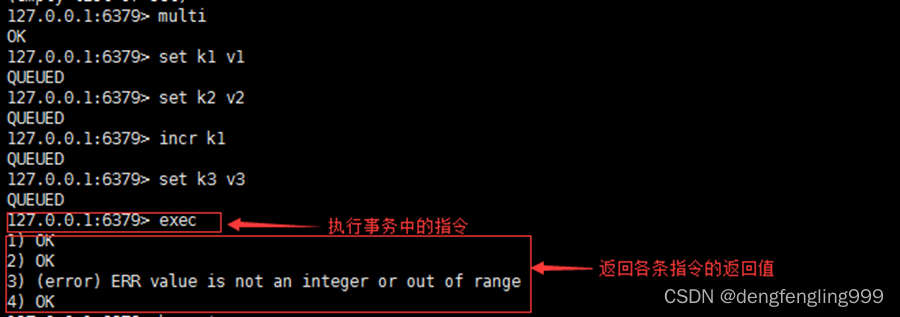
- A complete tutorial for getting started with redis: hyperloglog
- Set up a website with a sense of ceremony, and post it to 1/2 of the public network through the intranet
- [Jianzhi offer] 6-10 questions
- How to choose a securities company? Is it safe to open an account on your mobile phone
- phpcms付费阅读功能支付宝支付
- 【ODX Studio编辑PDX】-0.3-如何删除/修改Variant变体中继承的(Inherited)元素
- Redis入门完整教程:有序集合详解
- Basic knowledge of database
- Tweenmax emoticon button JS special effect
- Principle of lazy loading of pictures
猜你喜欢

随机推荐
[Jianzhi offer] 6-10 questions
Redis démarrer le tutoriel complet: Pipeline
[Taichi] change pbf2d (position based fluid simulation) of Taiji to pbf3d with minimal modification
【taichi】用最少的修改将太极的pbf2d(基于位置的流体模拟)改为pbf3d
Sword finger offer 67 Convert a string to an integer
Header file duplicate definition problem solving "c1014 error“
Feature scaling normalization
Redis入门完整教程:集合详解
【爬虫】数据提取之JSONpath
PICT 生成正交测试用例教程
C语言快速解决反转链表
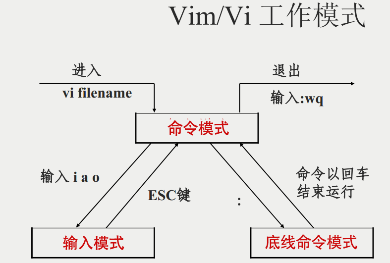
VIM editor knowledge summary
On-off and on-off of quality system construction
Analysis of the self increasing and self decreasing of C language function parameters
ETCD数据库源码分析——处理Entry记录简要流程
CTF竞赛题解之stm32逆向入门
刷题指南-public
[sword finger offer] questions 1-5
Principle of lazy loading of pictures
A complete tutorial for getting started with redis: redis usage scenarios