Tensorflow—Image segmentation

explain ： This article is for the author to learn Tensorflow Study notes during the official tutorial , Now it is sorted out for your reference . You can read and learn this article as the Chinese translation of the official tutorial . The code of this tutorial is consistent with the official code .

Tensorflow The official tutorial ¹ The link is attached at the end of the article .

Image segmentation

What is image segmentation ？

Image segmentation is a key process in computer vision . It includes segmenting visual input into segments to simplify image analysis . A fragment represents a target or part of a target , And by pixel set or “ Super pixel ” form . Image segmentation organizes pixels into larger parts , Eliminates the need to use a single pixel as an observation unit .

The task of image segmentation is to train a neural network to output the pixel range mask of the image . This can help us at a lower level （ Such as pixel hierarchy ） To understand the image .

Image segmentation is widely used in medical imaging 、 Autopilot 、 Satellite imaging .

This tutorial will use Oxford-IIIT Pet Data sets , This data set contains labels and pixel masks of pictures . The mask is the basic label of each pixel .

Each pixel contains one of the following three ：

• Class 1： Pixels belonging to pets
• Class 2： Pet pixel boundary
• Class 3： Not including the above / Surround pixels

The import module

pip install git+https://github.com/tensorflow/examples.git

import tensorflow as tf

from tensorflow_examples.models.pix2pix import pix2pix

import tensorflow_datasets as tfds

from IPython.display import clear_output
import matplotlib.pyplot as plt

Start

download Oxford-IIIT Pets Data sets & Preprocessing

The data set already contains the required data . The split mask is included in the version 3 And above .

dataset, info = tfds.load('oxford_iiit_pet:3.*.*', with_info=True)

The following code enhances our data by flipping the image

• The pixels in the segmentation mask have been marked {1, 2, 3}, For convenience , We will subtract the marks in the split mask 1, The new label result is {0, 1, 2};

def normalize(input_image, input_mask):   # Standardized images 
  input_image = tf.cast(input_image, tf.float32) / 255.0
  input_mask -= 1
  return input_image, input_mask

@tf.function
def load_image_train(datapoint):
  input_image = tf.image.resize(datapoint['image'], (128, 128))
  input_mask = tf.image.resize(datapoint['segmentation_mask'], (128, 128))

  if tf.random.uniform(()) > 0.5:
    input_image = tf.image.flip_left_right(input_image)
    input_mask = tf.image.flip_left_right(input_mask)

  input_image, input_mask = normalize(input_image, input_mask)

  return input_image, input_mask

def load_image_test(datapoint):
  input_image = tf.image.resize(datapoint['image'], (128, 128))
  input_mask = tf.image.resize(datapoint['segmentation_mask'], (128, 128))

  input_image, input_mask = normalize(input_image, input_mask)

  return input_image, input_mask

The dataset already contains the required separation of testing and training , Next we continue to use the same separation .

TRAIN_LENGTH = info.splits['train'].num_examples
BATCH_SIZE = 64
BUFFER_SIZE = 1000
STEPS_PER_EPOCH = TRAIN_LENGTH // BATCH_SIZE

train = dataset['train'].map(load_image_train, num_parallel_calls=tf.data.AUTOTUNE)
test = dataset['test'].map(load_image_test)

train_dataset = train.cache().shuffle(BUFFER_SIZE).batch(BATCH_SIZE).repeat()
train_dataset = train_dataset.prefetch(buffer_size=tf.data.AUTOTUNE)
test_dataset = test.batch(BATCH_SIZE)

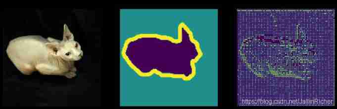
Next, we let the image in the dataset and the corresponding mask display on the screen .

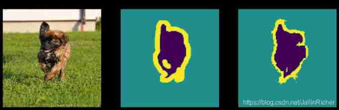
def display(display_list):
  plt.figure(figsize=(15, 15))

  title = ['Input Image', 'True Mask', 'Predicted Mask']

  for i in range(len(display_list)):
    plt.subplot(1, len(display_list), i+1)
    plt.title(title[i])
    plt.imshow(tf.keras.preprocessing.image.array_to_img(display_list[i]))
    plt.axis('off')
  plt.show()

for image, mask in train.take(1):
  sample_image, sample_mask = image, mask
display([sample_image, sample_mask])

Defining models

The model we use is an improved U-Net.U-Net By encoder （ Lower sampler ） And decoder .

A pre trained model is used as an encoder , Make the network learn robust features , And reduce the number of parameters that can be trained .

We use the trained MobileNetV2 Model as encoder , We will use its intermediate output .

The decoder will use Tensorflow Examples Medium Pix2pix The upper sampler that has been implemented in the tutorial .

OUTPUT_CHANNELS = 3

Because each pixel has three labels , So our output channel is set to 3

MobileNetV2 Model we can use tf.keras.applications To call . The encoder is composed of special outputs of the middle layer of the model . Note that the encoder will not be trained during model training .

base_model = tf.keras.applications.MobileNetV2(input_shape=[128, 128, 3], include_top=False)

# Use the activations of these layers
layer_names = [
    'block_1_expand_relu',   # 64x64
    'block_3_expand_relu',   # 32x32
    'block_6_expand_relu',   # 16x16
    'block_13_expand_relu',  # 8x8
    'block_16_project',      # 4x4
]
base_model_outputs = [base_model.get_layer(name).output for name in layer_names]

# Create the feature extraction model
down_stack = tf.keras.Model(inputs=base_model.input, outputs=base_model_outputs)

down_stack.trainable = False

Encoder is a series that has been in Tensorflow Examples Upper sampler implemented in .

up_stack = [
    pix2pix.upsample(512, 3),  # 4x4 -> 8x8
    pix2pix.upsample(256, 3),  # 8x8 -> 16x16
    pix2pix.upsample(128, 3),  # 16x16 -> 32x32
    pix2pix.upsample(64, 3),   # 32x32 -> 64x64
]

def unet_model(output_channels):
  inputs = tf.keras.layers.Input(shape=[128, 128, 3])

  # Downsampling through the model
  skips = down_stack(inputs)
  x = skips[-1]
  skips = reversed(skips[:-1])

  # Upsampling and establishing the skip connections
  for up, skip in zip(up_stack, skips):
    x = up(x)
    concat = tf.keras.layers.Concatenate()
    x = concat([x, skip])

  # This is the last layer of the model
  last = tf.keras.layers.Conv2DTranspose(
      output_channels, 3, strides=2,
      padding='same')  #64x64 -> 128x128

  x = last(x)

  return tf.keras.Model(inputs=inputs, outputs=x)

Training models

Now let's compile and train the model . We will use losses.SparseCategoricalCrossentropy(from_logits=True) Loss function . Because the network will be like multi category prediction , Assign a label to each pixel .

In the actual separation mask , Every pixel will have {0, 1, 2} Three labels . The network will output three channels . Essentially , Each channel learns to predict a category , And the loss function is the recommended function of this kind of scheme .

Use the output of the network , The label assigned to the pixel represents the channel with the highest value .

model = unet_model(OUTPUT_CHANNELS)
model.compile(optimizer='adam',
              loss=tf.keras.losses.SparseCategoricalCrossentropy(from_logits=True),
              metrics=['accuracy'])

Take a quick look at the structure of the result model ：

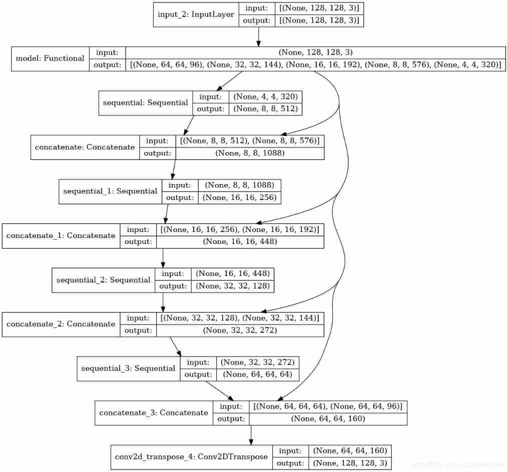
tf.keras.utils.plot_model(model, show_shapes=True)

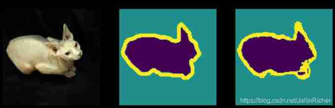
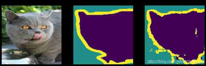
Test the model to see what it predicts before training ：

def create_mask(pred_mask):
  pred_mask = tf.argmax(pred_mask, axis=-1)
  pred_mask = pred_mask[..., tf.newaxis]
  return pred_mask[0]

def show_predictions(dataset=None, num=1):
  if dataset:
    for image, mask in dataset.take(num):
      pred_mask = model.predict(image)
      display([image[0], mask[0], create_mask(pred_mask)])
  else:
    display([sample_image, sample_mask,
             create_mask(model.predict(sample_image[tf.newaxis, ...]))])

show_predictions()

Start training

Let's observe how the model improves during training . To complete this character , Let's define a return function ：

class DisplayCallback(tf.keras.callbacks.Callback):
  def on_epoch_end(self, epoch, logs=None):
    clear_output(wait=True)
    show_predictions()
    print ('\nSample Prediction after epoch {}\n'.format(epoch+1))

EPOCHS = 20
VAL_SUBSPLITS = 5
VALIDATION_STEPS = info.splits['test'].num_examples//BATCH_SIZE//VAL_SUBSPLITS

model_history = model.fit(train_dataset, epochs=EPOCHS,
                          steps_per_epoch=STEPS_PER_EPOCH,
                          validation_steps=VALIDATION_STEPS,
                          validation_data=test_dataset,
                          callbacks=[DisplayCallback()])

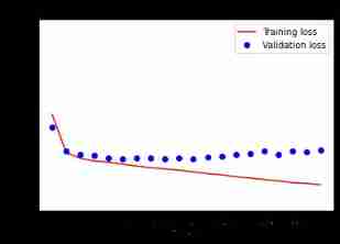
loss = model_history.history['loss']
val_loss = model_history.history['val_loss']

plt.figure()
plt.plot(model_history.epoch, loss, 'r', label='Training loss')
plt.plot(model_history.epoch, val_loss, 'bo', label='Validation loss')
plt.title('Training and Validation Loss')
plt.xlabel('Epoch')
plt.ylabel('Loss Value')
plt.ylim([0, 1])
plt.legend()
plt.show()

Start to predict

• To save time , We continue to use smaller epochs, But if you want to get more accurate results, you can turn it up .

show_predictions(test_dataset, 3)

end

---

---

---

optional ： Unbalanced classes and class weights

If you are interested, please refer to the official tutorial

---

---

---

---

1. The official tutorial ︎