当前位置:网站首页>2021 Li Hongyi machine learning (3): what if neural network training fails
2021 Li Hongyi machine learning (3): what if neural network training fails
2022-07-05 02:39:00 【Three ears 01】
2021 Li hongyi machine learning (3): What if the neural network can't be trained
1 Mission Introduction
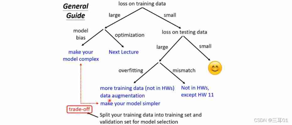
1.1 If on the training set loss Always not small enough
- Situation 1 :model bias( The model itself has great limitations )—— Build more complex models
- Situation two : optimization problem ( The optimization method used cannot be optimized to loss minimum value )—— More effective optimization methods
How to judge what kind of situation ?
- First, train on a shallow network that is easier to optimize
- If the deep network cannot get smaller than the above on the training set loss, It is case two
1.2 If loss On the training set , On the test set
- Situation 1 :overfitting—— The simplest solution is to add training data Data augmentation:

The original data can be processed , Get new data that can be added to the training set : The first picture above is the original , second 、 The three pictures are the inversion and local enlargement of the original picture . And the fourth picture is the picture upside down , This makes model recognition more difficult , So the method of the fourth picture is not good .
The second method is to add restrictions to the model , For example, the model must be a conic , But be careful not to limit too much .
How to select a model ?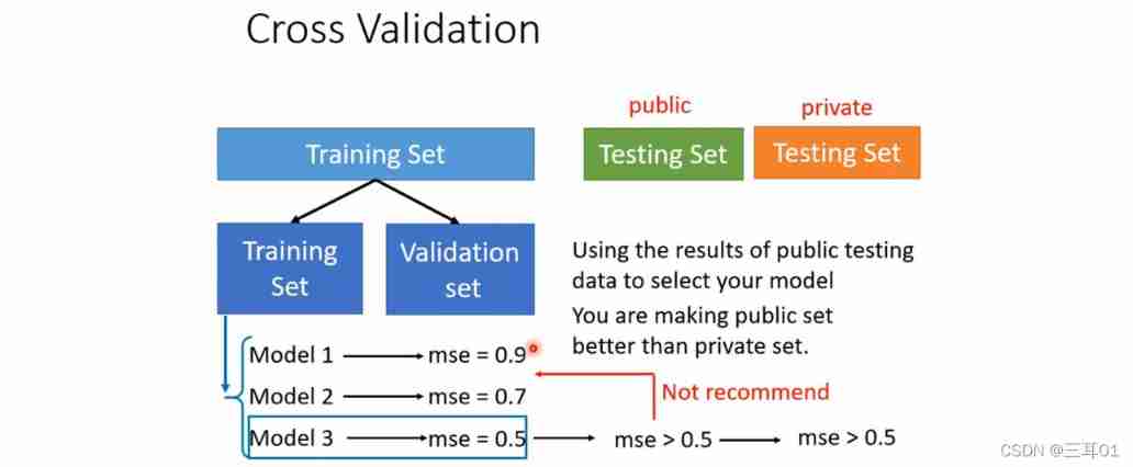
- Situation two :mismatch
overfitting It can be solved by adding the data of the training set , however mismatch Of training and testing Different distribution of , It can't be solved like that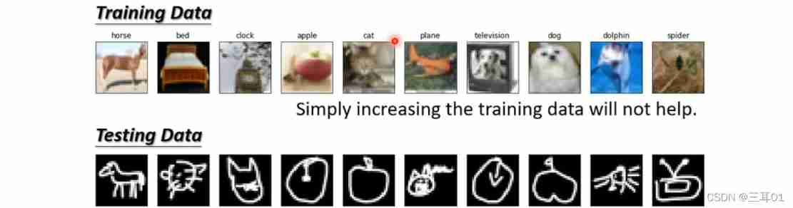
1.3 Schematic diagram of mission strategy
2 Local minimum (local minima) And saddle point (saddle point)
When loss When unable to descend , Maybe the gradient is close 0 了 , This is a , Local minimum (local minima) And saddle point (saddle point) It's possible , They are collectively referred to as critical point.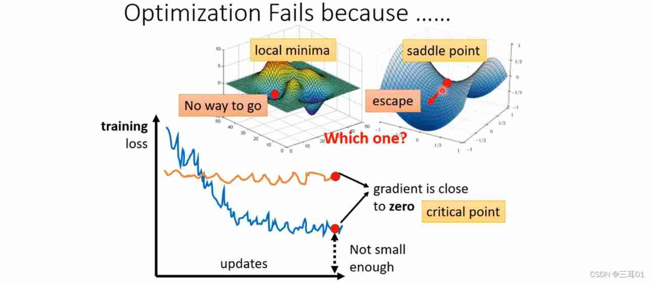
here , We need to judge which situation it belongs to , Calculation Hessian that will do :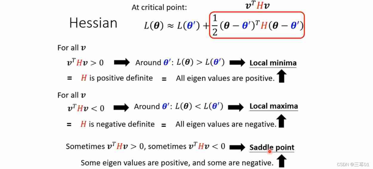
give an example :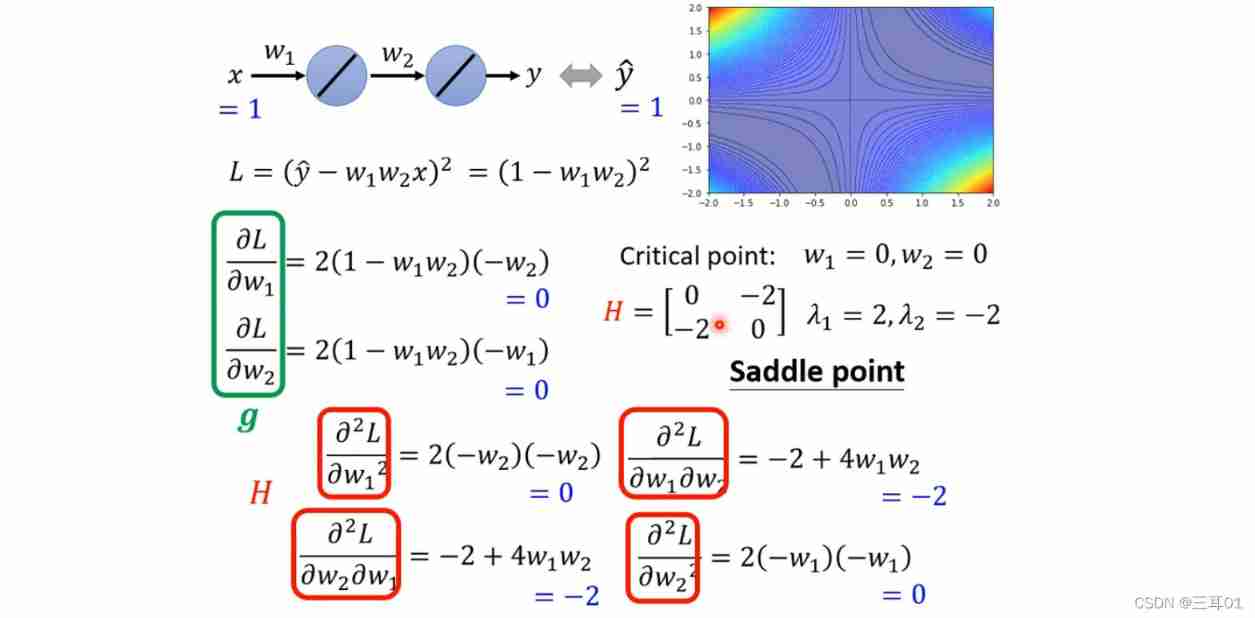
If it's a saddle point (saddle point), You can also find the direction of descent and continue training .
But in fact, this kind of situation is rare .
3 batch (batch) And momentum (momentum)
3.1 batch (batch)
Small batch size Have better results .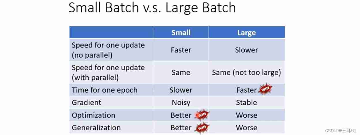
There are many articles that want to have it both ways :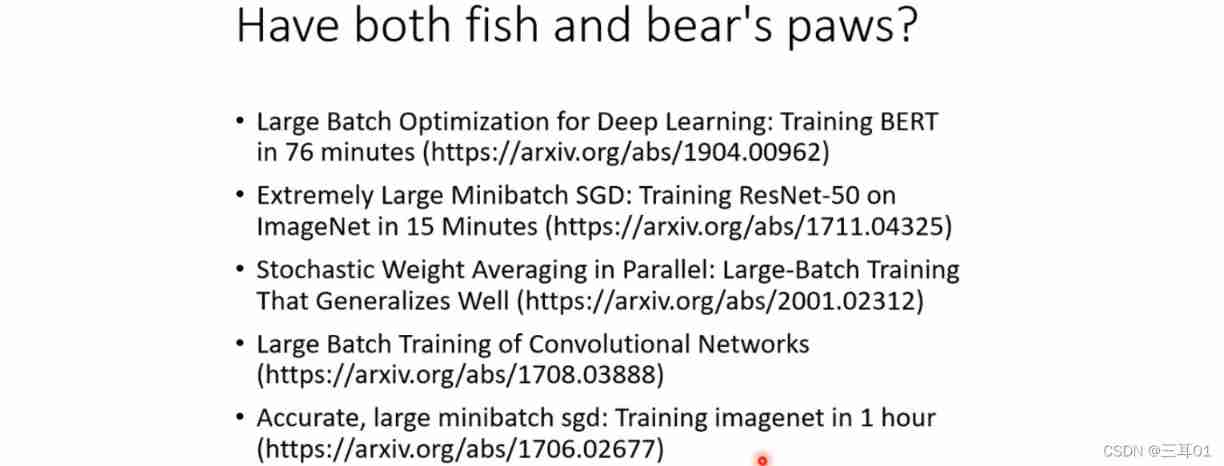
3.2 momentum (momentum)
With momentum , Will not stay in critical point, But will continue down :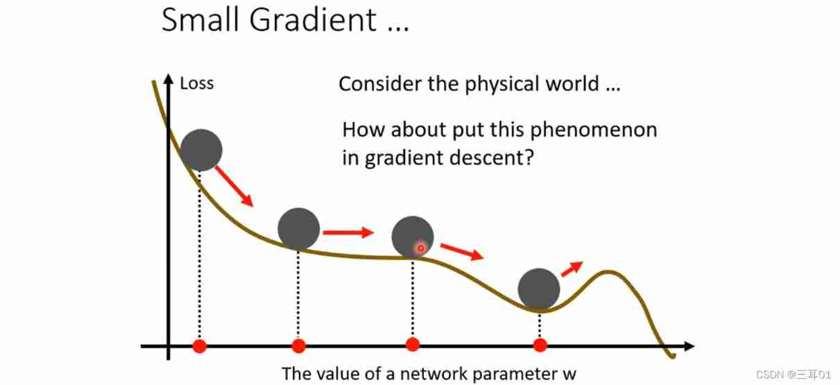
The previous gradient descent is like this :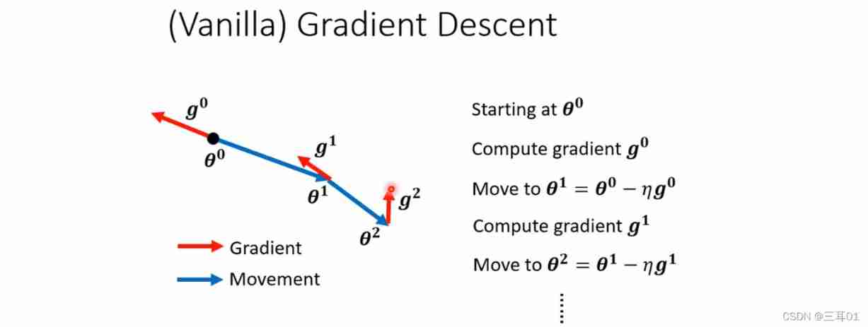
After adding momentum , Is to add the consideration of the previous action , Then the next action is the result of the combination of the previous action and the previous action .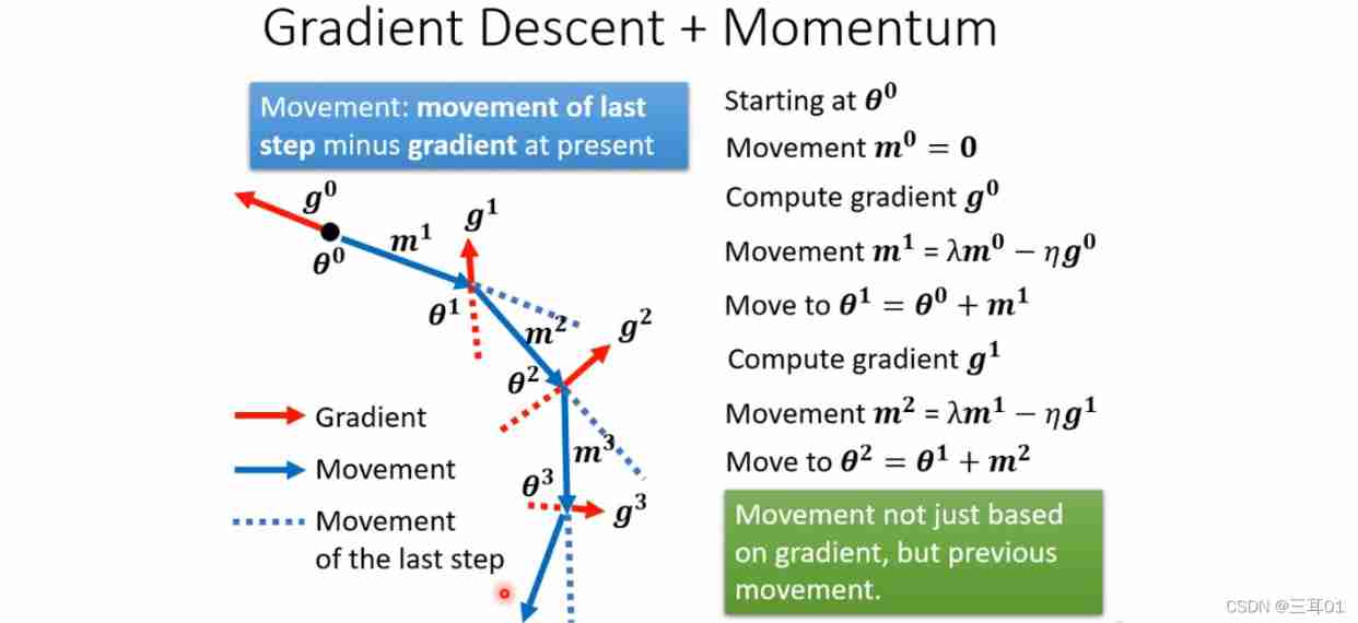
The red line below is the gradient , The blue dotted line is momentum , The blue solid line is the result of the combination of the first two , You can see , Maybe even climb over the hill , Reach the real loss minimum value .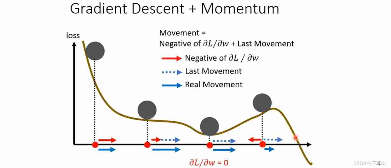
4 Automatically adjust the learning rate (Learning Rate)
In the front loss When not falling , We said it might be critical point, But it may also be the following :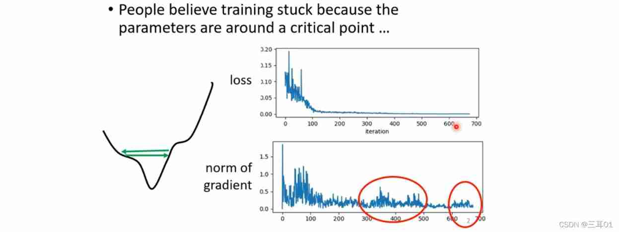
learning rate It should be customized for each parameter :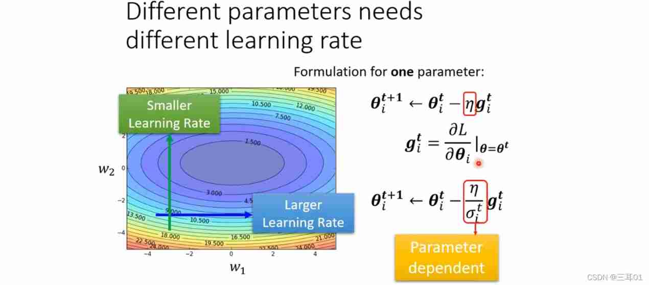
Number of original parameters t + 1 t+1 t+1 In the next iteration , Learning rate η \eta η It is the same. ; And after we modify , η \eta η Turned into η σ i t \frac{\eta}{\sigma^t_i} σitη, After this modification , The learning rate is parameter independent Of course. , It's also iteration independent Of ( Parameter independent 、 Iterative independence ).
4.1 The most common way to modify the learning rate is the root mean square
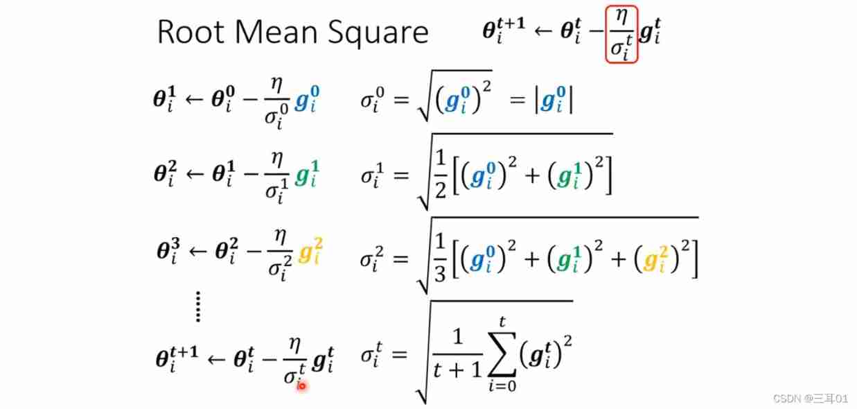
This method is used in Adagrad Inside :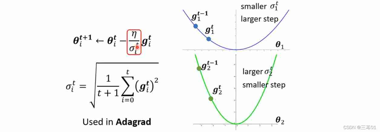
When the gradient is small , Calculated σ i t \sigma^t_i σit Just small , Then the learning rate is large ; On the contrary, the learning rate becomes smaller .
4.2 You can adjust your current gradient Importance ——RMSProp
This method is achieved by setting α \alpha α To adjust the importance of the current gradient :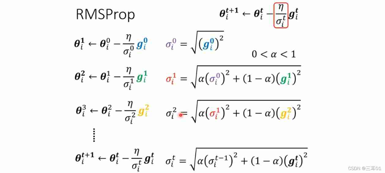
As shown in the figure below :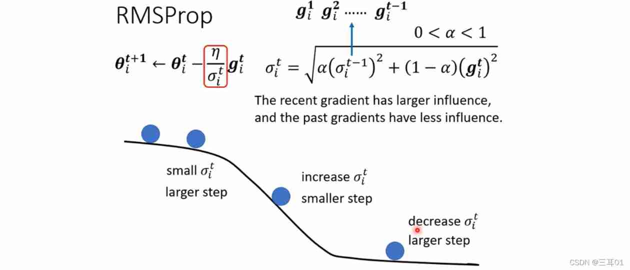
You can adjust α \alpha α The relatively small , Give Way σ i t \sigma^t_i σit More dependent g i t g^t_i git, such , When the gradient suddenly changes from smooth to steep , g i t g^t_i git Bigger , σ i t \sigma^t_i σit It's getting bigger , It will make the pace at this time smaller ; Empathy , When the gradient turns smooth again , σ i t \sigma^t_i σit Will quickly become smaller , The pace will get bigger .
In fact, it is to make every step react quickly according to the changing situation .
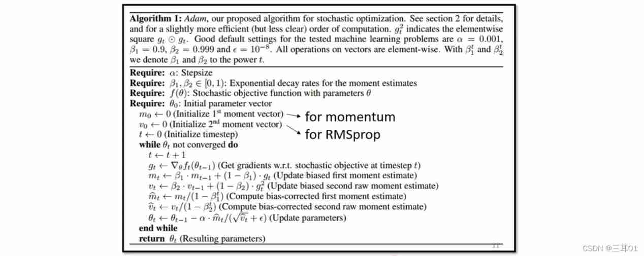
4.3 Adam: RMSProp + Momentum
4.4 Learning Rate Scheduling
Make learning rate η \eta η Over time :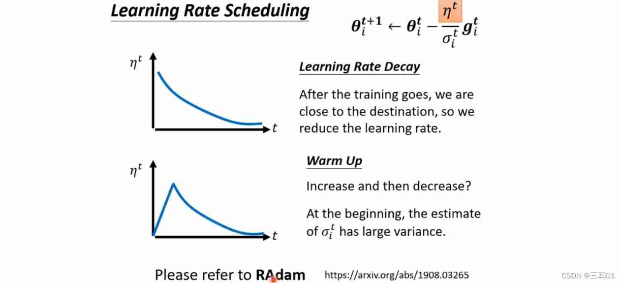
4.5 summary
Add the front 3.2, We use three methods to improve gradient descent : momentum 、 Adjust the learning rate 、 The learning rate changes over time .
m i t m^t_i mit and σ i t \sigma^t_i σit Will not offset each other , because m i t m^t_i mit Including the direction , and σ i t \sigma^t_i σit Only in size .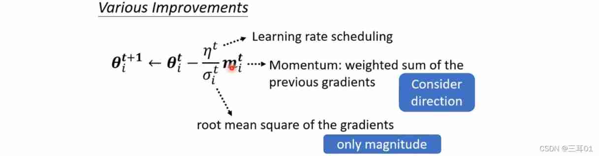
5 Loss function (Loss) It may also have an impact
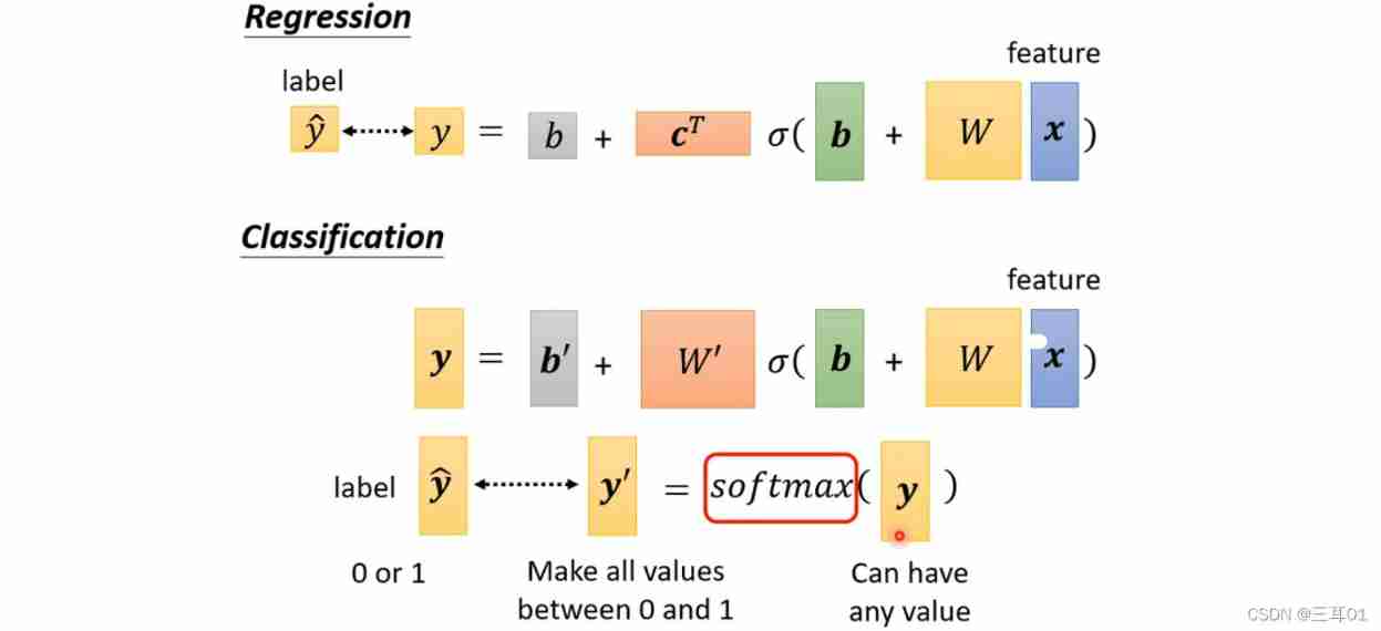
In classification , It's usually added softmax: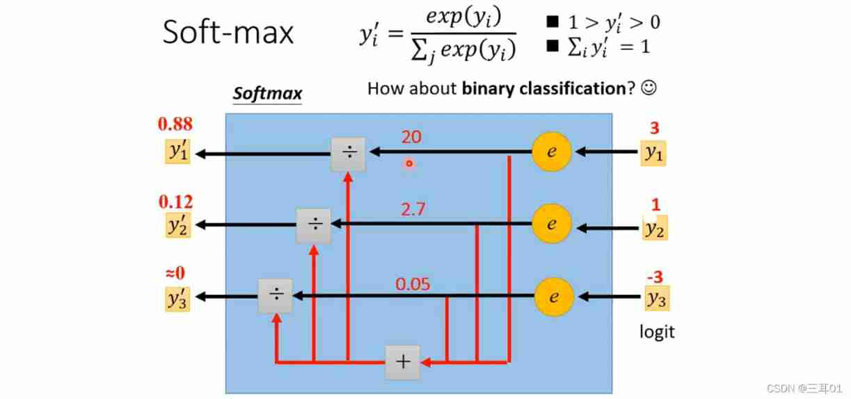
If it is classified into two categories , Is more commonly used sigmoid, But in fact, the results of these two methods are the same .
Here is the loss function :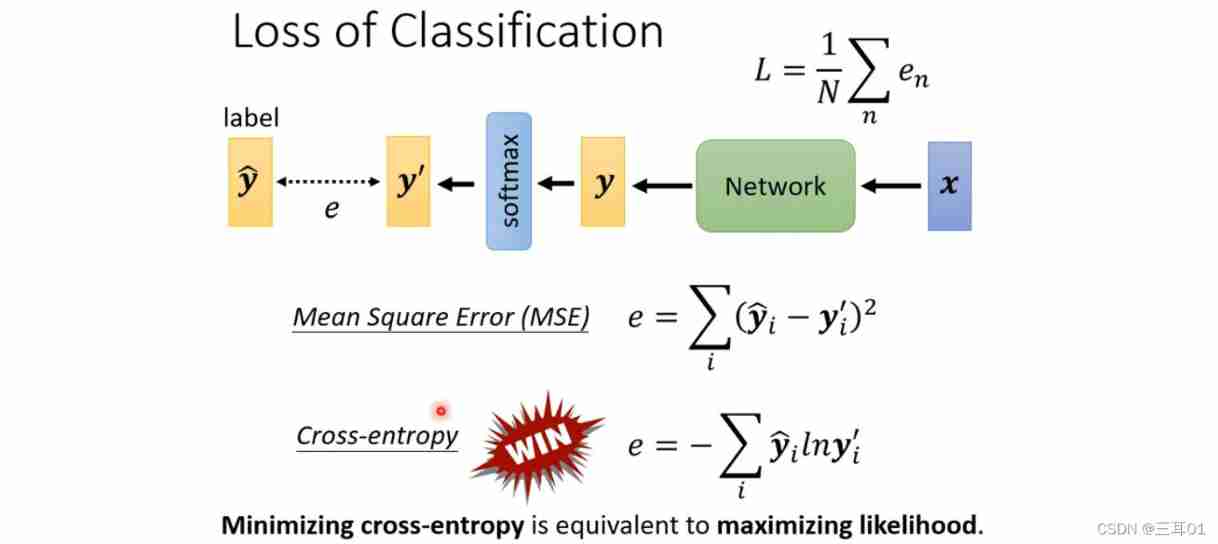
in fact , Cross entropy in classification is The most commonly used Of , stay PyTorch in ,CrossEntropyLoss This function already contains softmax, The two are bound together .
Why? ?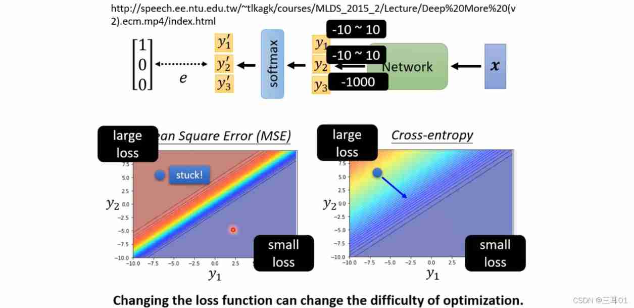
As you can see from the diagram , When loss When a large ,MSE Very flat , Cannot gradient down to loss A small place , Get stuck ; But the cross entropy can decline all the way .
6 Batch standardization (Batch Normalization)
Hope for different parameters , Yes loss The scope of influence is relatively uniform , Like the right figure below :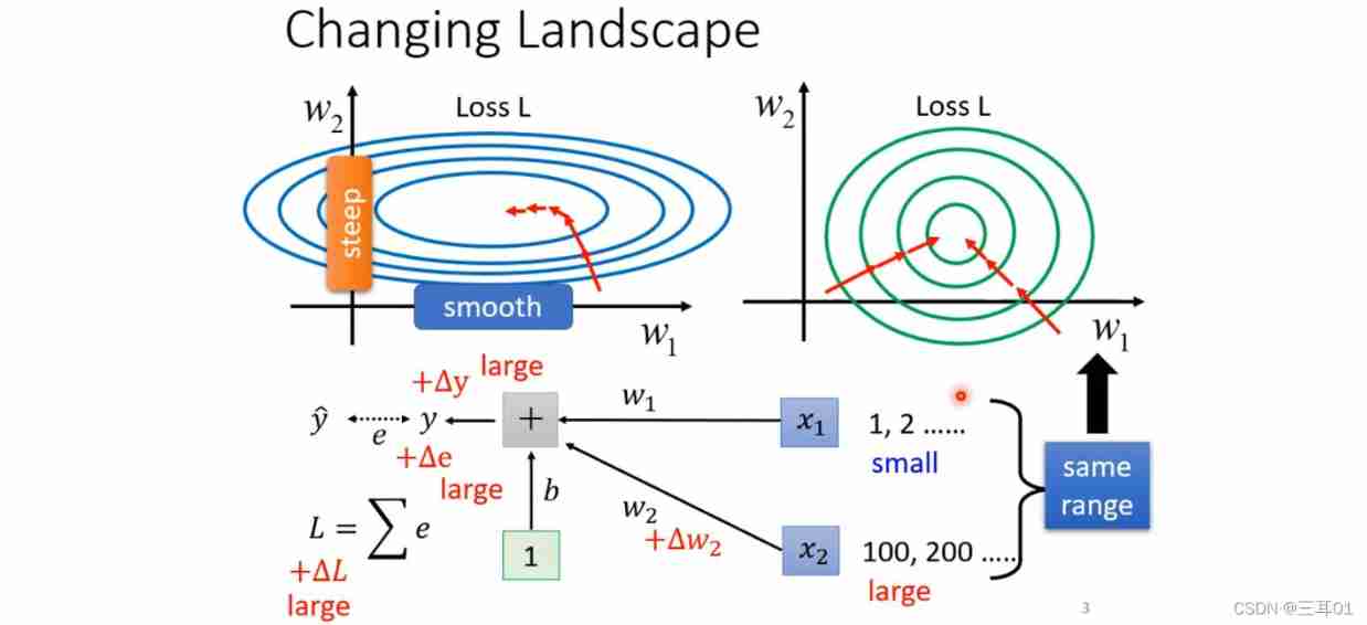
The method is feature normalization (Feature Normalization):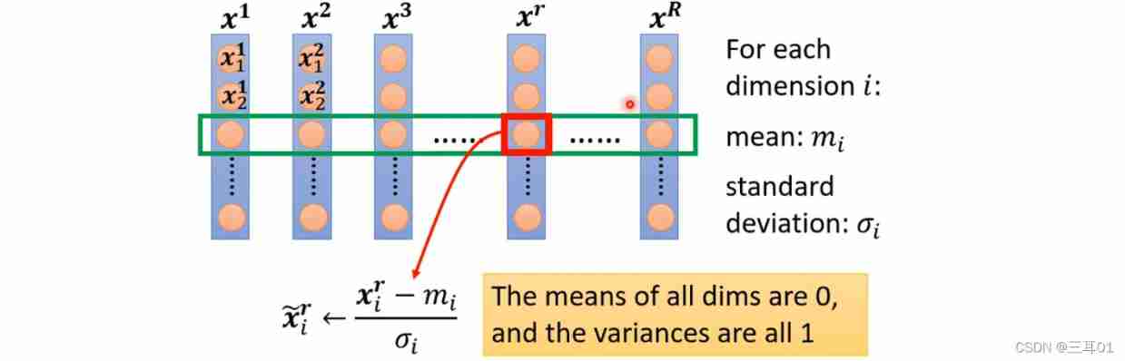
After normalization , The average value of the characteristics of each dimension is 0, The variance of 1.
Generally speaking , Feature normalization makes gradient descent converge faster .
The output of the next step also needs to be normalized , These normalization are aimed at a Batch Of :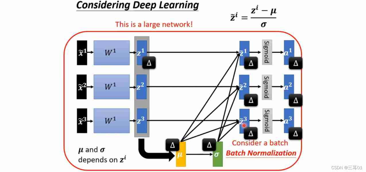
In order to make the mean value of the output not 0, The variance is not 1, It will add β \beta β and γ \gamma γ: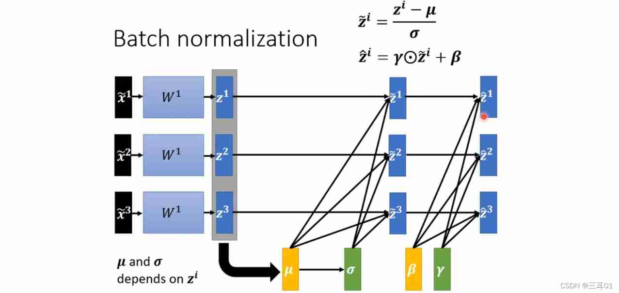
β \beta β and γ \gamma γ The initial values of these two vectors are 0 and 1, Then learn and update in the network step by step , So at the beginning ,dimension The distribution of is close , follow-up error surface After performing better , That's what makes β \beta β and γ \gamma γ add .
stay Testing in : take train Parameters of are used in test in .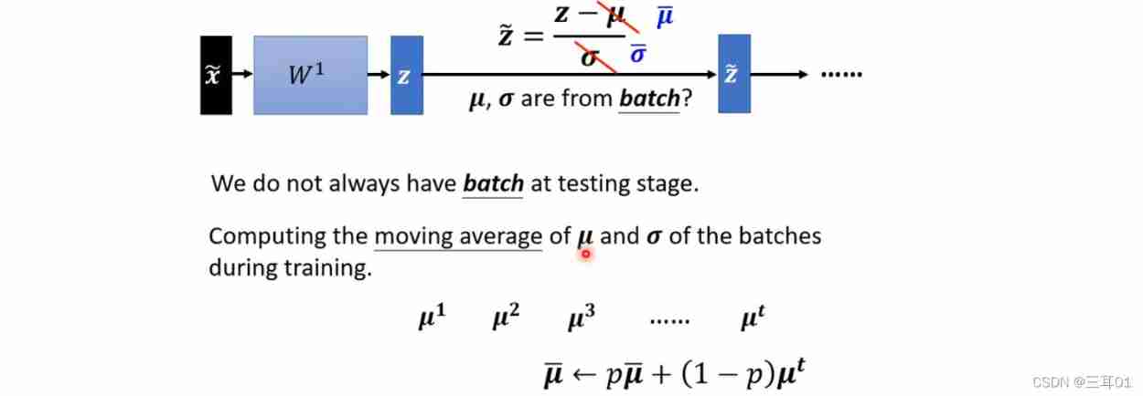
Some famous Normalization:
边栏推荐
- Why do you understand a16z? Those who prefer Web3.0 Privacy Infrastructure: nym
- When the low alcohol race track enters the reshuffle period, how can the new brand break the three major problems?
- ELFK部署
- Hmi-30- [motion mode] the module on the right side of the instrument starts to write
- Application and Optimization Practice of redis in vivo push platform
- Vb+access hotel service management system
- 8. Commodity management - commodity classification
- Medusa installation and simple use
- [機緣參悟-38]:鬼穀子-第五飛箝篇 - 警示之一:有一種殺稱為“捧殺”
- Elk log analysis system
猜你喜欢
Write a thread pool by hand, and take you to learn the implementation principle of ThreadPoolExecutor thread pool
Naacl 2021 | contrastive learning sweeping text clustering task
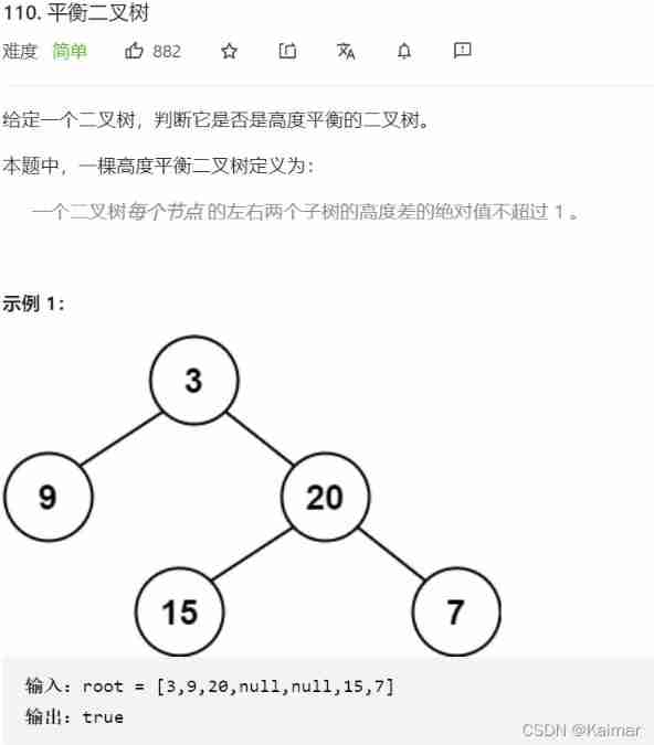
【LeetCode】110. Balanced binary tree (2 brushes of wrong questions)

The perfect car for successful people: BMW X7! Superior performance, excellent comfort and safety

Can you really learn 3DMAX modeling by self-study?
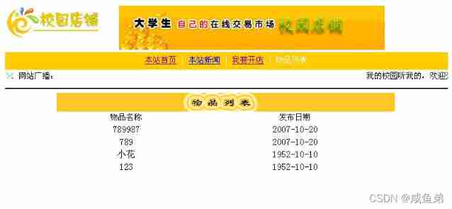
Asp+access campus network goods trading platform
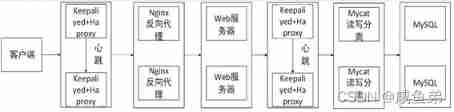
Design and implementation of high availability website architecture

A tab Sina navigation bar
【LeetCode】111. Minimum depth of binary tree (2 brushes of wrong questions)
![[download white paper] does your customer relationship management (CRM) really](/img/e3/f130d071afb7309fdbf8a9c65b1d38.jpg)
[download white paper] does your customer relationship management (CRM) really "manage" customers?
随机推荐
[機緣參悟-38]:鬼穀子-第五飛箝篇 - 警示之一:有一種殺稱為“捧殺”
Write a thread pool by hand, and take you to learn the implementation principle of ThreadPoolExecutor thread pool
Leetcode takes out the least number of magic beans
[source code attached] Intelligent Recommendation System Based on knowledge map -sylvie rabbit
The most powerful new household god card of Bank of communications. Apply to earn 2100 yuan. Hurry up if you haven't applied!
Elk log analysis system
Last week's hot review (2.7-2.13)
Grub 2.12 will be released this year to continue to improve boot security
[uc/os-iii] chapter 1.2.3.4 understanding RTOS
RichView TRVUnits 图像显示单位
From task Run get return value - getting return value from task Run
Asp+access campus network goods trading platform
Design of KTV intelligent dimming system based on MCU
Erreur de type de datagramme MySQL en utilisant Druid
Redis distributed lock, lock code logic
【微服务|SCG】Filters的33种用法
Introduce reflow & repaint, and how to optimize it?
February database ranking: how long can Oracle remain the first?
[机缘参悟-38]:鬼谷子-第五飞箝篇 - 警示之一:有一种杀称为“捧杀”
Official announcement! The third cloud native programming challenge is officially launched!