PyTorch nn. Full analysis of RNN parameters

One 、 brief introduction

torch.nn.RNN Used to build circular layers , The calculation rules are as follows ：

$${\mathbf{h}}_t=\tanh ({\mathbf{W}}_{ih}{\mathbf{x}}_t+{\mathbf{b}}_{ih}+{\mathbf{W}}_{hh}{\mathbf{h}}_{t-1}+{\mathbf{b}}_{hh})\text{\hspace{1em}(1)}$$

among ${\mathbf{h}}_t$ yes $t$ The hidden state of the moment ,${\mathbf{x}}_t$ yes $t$ Time input . Subscript $i$ yes $input$ Abbreviation , Subscript $h$ yes $hidden$ Abbreviation .$\mathbf{W},\mathbf{b}$ They are weight and offset .

Two 、 Pre knowledge

First, let's review the general neural network , We usually feed a small batch of data in the process of training it . Might as well set $\text{batch\_size}=N$, The form of feeding data is ：

$$\mathbf{X}={\left[\begin{array}{c}{\mathbf{x}}_1^{\text{T}}\\ ⋮\\ {\mathbf{x}}_N^{\text{T}}\end{array}\right]}_{N\times d}$$

among ${\mathbf{x}}_i=(x_{i1},x_{i2},\cdots ,x_{id}{)}^{\text{T}}$ Is the eigenvector , Dimension is $d$.

In dealing with sequence problems , We will transform the lexical elements into corresponding eigenvectors . For example, when dealing with an English sentence , We usually transform each word into an appropriate feature vector by some means . Let's set the sequence （ The sentence ） The length is $L$, So in this scenario , A sentence can be expressed as ：

$${\text{seq}}_i={\left[\begin{array}{c}{\mathbf{x}}_{i1}^{\text{T}}\\ ⋮\\ {\mathbf{x}}_{iL}^{\text{T}}\end{array}\right]}_{L\times d}$$

Each of them ${\mathbf{x}}_{ij},j=1,\cdots ,L$ They all correspond to sentences ${\text{seq}}_i$ One of the words in . Under the above agreement , We stay $t$ moment Feed to RNN The data is ：

$${\mathbf{X}}_t={\left[\begin{array}{c}{\mathbf{x}}_{1t}^{\text{T}}\\ ⋮\\ {\mathbf{x}}_{Nt}^{\text{T}}\end{array}\right]}_{N\times d}\text{\hspace{1em}(2)}$$

thus $(1)$ The formula is rewritten as

$${\mathbf{H}}_t=\tanh ({\mathbf{X}}_t{\mathbf{W}}_{ih}+{\mathbf{b}}_{ih}+{\mathbf{H}}_{t-1}{\mathbf{W}}_{hh}+{\mathbf{b}}_{hh})\text{\hspace{1em}(3)}$$

among ${\mathbf{H}}_t,{\mathbf{H}}_{t-1}$ The shape of is $N\times h$,${\mathbf{W}}_{ih}$ The shape of is $d\times h$,${\mathbf{W}}_{hh}$ The shape of is $h\times h$,${\mathbf{b}}_{ih},{\mathbf{b}}_{hh}$ The shape of is $1\times h$, The broadcast mechanism is used when summing .

stay nn.RNN in , We feed all the data at all times at one time , The data is in the form of ：

$$\mathbf{X}=[{\text{seq}}_1,{\text{seq}}_2,\cdots ,{\text{seq}}_N{]}_{N\times L\times d}\text{or}\mathbf{X}=[{\mathbf{X}}_1,{\mathbf{X}}_2,\cdots ,{\mathbf{X}}_L{]}_{L\times N\times d}$$

The left side represents batch_first=True The circumstances of , The right represents batch_first=False The circumstances of .

Be careful ： In a batch in , all sequence Keep the same length , namely $L$ Need to be consistent .

3、 ... and 、 analysis

3.1 All the parameters

With pre knowledge , We can easily explain these parameters .

• input_size： namely $d$;
• hidden_size： namely $h$;
• num_layers： namely RNN The number of layers . The default is $1$ layer . This parameter is greater than $1$ when , Will form the Stacked RNN, Also called multilayer RNN Or depth RNN;
• nonlinearity： That is, the nonlinear activation function . You can choose tanh or relu, The default is tanh;
• bias： Offset . Enabled by default , Can choose to close ;
• batch_first： That is, whether to choose to let batch_size As the first parameter in the input shape . When batch_first=True when , Input should have $N\times L\times d$ This shape , Otherwise, it should have $L\times N\times d$ This shape . The default is False;
• dropout： That is, whether to enable dropout. To enable , You should set dropout Probability , At this time, except for the last floor ,RNN One will be added at the back of each floor dropout layer . The default is $0$, That is, do not enable ;
• bidirectional： That is, whether to enable bidirectional RNN, Off by default .

3.2 Input parameters

Here we only consider batch The situation of .

When batch_first=True when , Input input Should have shape $N\times L\times d$, Otherwise it should have shape $L\times N\times d$.

h_0 Is the implicit state at the initial time . When RNN It is unidirectional RNN when ,h_0 The shape of the should be $\text{num\_layers}\times N\times h$; When RNN It's two-way RNN when ,h_0 The shape of the should be $(2\cdot \text{num\_layers})\times N\times h$. If the value of this parameter is not provided , The default is all 0 tensor .

3.3 Output parameters

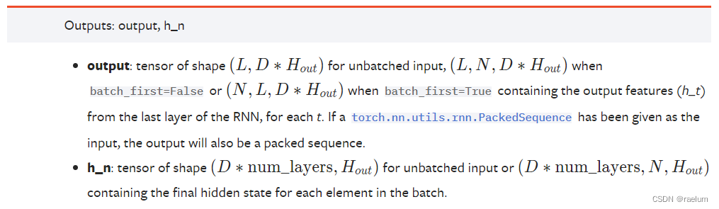
Here we only consider batch The situation of .

When RNN It is unidirectional RNN when ： if batch_first=True, Output output Having shape $N\times L\times h$, Otherwise, it has a shape $L\times N\times h$. When batch_first=False when ,output[t, :, :] Represents the moment $t$ when ,RNN The last layer （ The term "last layer" is used because it may appear Stacked RNN situation ） Output ${\mathbf{h}}_t$.h_n Represents the final implicit state , Shape is $\text{num\_layers}\times N\times h$.

When RNN It's two-way RNN when ： if batch_first=True, Output output Having shape $N\times L\times 2h$, Otherwise, it has a shape $L\times N\times 2h$.h_n The shape of is $(2\cdot \text{num\_layers})\times N\times h$.

in fact , For unidirectional RNN, Yes

$$\text{output}=[{\mathbf{H}}_1,{\mathbf{H}}_2,\cdots ,{\mathbf{H}}_L{]}_{L\times N\times h},\text{h\_n}=[{\mathbf{H}}_L{]}_{1\times N\times h}$$

Four 、 Further understand through examples nn.RNN

One way with a single hidden layer RNN For example （ The following examples all default batch_first=False）.

Suppose there is an English sentence ：He ate an apple., Ignore . And set the word element as word （word） when , The length of the sequence is $4$. For simplicity , Let's assume that each word element corresponds to a $6$ The eigenvectors of the dimensions , Then the above sequence can be written as ：

import torch
import torch.nn as nn

torch.manual_seed(42)
seq = torch.randn(4, 6)  #  Just for example 
print(seq)
# tensor([[ 1.9269, 1.4873, 0.9007, -2.1055, 0.6784, -1.2345],
# [-0.0431, -1.6047, 0.3559, -0.6866, -0.4934, 0.2415],
# [-1.1109, 0.0915, -2.3169, -0.2168, -0.3097, -0.3957],
# [ 0.8034, -0.6216, -0.5920, -0.0631, -0.8286, 0.3309]])

Think of this sentence as a batch, namely （ Note that the shape is $L\times N\times d$）：

inputs = seq.unsqueeze(1)
print(inputs)
# tensor([[[ 1.9269, 1.4873, 0.9007, -2.1055, 0.6784, -1.2345]],
# [[-0.0431, -1.6047, 0.3559, -0.6866, -0.4934, 0.2415]],
# [[-1.1109, 0.0915, -2.3169, -0.2168, -0.3097, -0.3957]],
# [[ 0.8034, -0.6216, -0.5920, -0.0631, -0.8286, 0.3309]]])
print(inputs.shape)
# torch.Size([4, 1, 6])

With inputs, We also need to initialize the implicit state h_0, Might as well set $h=3$：

h_0 = torch.randn(1, 1, 3)
print(h_0)
# tensor([[[ 1.3525, 0.6863, -0.3278]]])

Next create RNN layer , In fact, you only need to input input_size and hidden_size that will do ：

rnn = nn.RNN(6, 3)

Observe the output ：

outputs, h_n = rnn(inputs, h_0)
print(outputs)
# tensor([[[-0.5428, 0.9207, 0.7060]],
# [[-0.2245, 0.2461, -0.4578]],
# [[ 0.5950, -0.3390, -0.4598]],
# [[ 0.9281, -0.7660, 0.5954]]], grad_fn=<StackBackward0>)
print(h_n)
# tensor([[[ 0.9281, -0.7660, 0.5954]]], grad_fn=<StackBackward0>)

5、 ... and 、 Write a single hidden layer one-way from scratch RNN

First write the frame ：

class RNN(nn.Module):

    def __init__(self, input_size, hidden_size):
        super().__init__()
        pass

    def forward(self, inputs, h_0):
        pass

Our calculations follow $(3)$ type , namely ：

$${\mathbf{H}}_t=\tanh ({\mathbf{X}}_t{\mathbf{W}}_{ih}+{\mathbf{b}}_{ih}+{\mathbf{H}}_{t-1}{\mathbf{W}}_{hh}+{\mathbf{b}}_{hh})$$

class RNN(nn.Module):

    def __init__(self, input_size, hidden_size):
        super().__init__()
        self.W_ih = torch.randn(input_size, hidden_size)
        self.W_hh = torch.randn(hidden_size, hidden_size)
        self.b_ih = torch.randn(1, hidden_size)
        self.b_hh = torch.randn(1, hidden_size)

    def forward(self, inputs, h_0):
        L, N, d = inputs.shape  #  Respectively corresponding to the sequence length 、 Lot size and feature dimension 
        H = h_0[0]  #  because h_0 The shape of is (1,N,h), We need to use (N,h) To calculate 
        outputs = []  #  Used to store h_1,h_2,...,h_L
        for t in range(L):
            X_t = inputs[t]
            H = torch.tanh(X_t @ self.W_ih + self.b_ih + H @ self.W_hh + self.b_hh)
            outputs.append(H)
        h_n = outputs[-1].unsqueeze(0)  # h_n It's actually h_L, But the shape at this time is (N,h)
        outputs = torch.cat(outputs, 0).unsqueeze(1)
        return outputs, h_n

To test our RNN That's right. , We need to use the same input to verify whether our output is consistent with the previous .

torch.manual_seed(42)
seq = torch.randn(4, 6)
inputs = seq.unsqueeze(1)
h_0 = torch.randn(1, 1, 3)

#  keep RNN Internal parameters ： Weight and offset are consistent 
rnn = nn.RNN(6, 3)
params = [param.data.T for param in rnn.parameters()]
my_rnn = RNN(6, 3)
my_rnn.W_ih = params[0]
my_rnn.W_hh = params[1]
my_rnn.b_ih[0] = params[2]
my_rnn.b_hh[0] = params[3]

outputs, h_n = my_rnn(inputs, h_0)
print(outputs)
# tensor([[[-0.5428, 0.9207, 0.7060]],
# [[-0.2245, 0.2461, -0.4578]],
# [[ 0.5950, -0.3390, -0.4598]],
# [[ 0.9281, -0.7660, 0.5954]]])
print(h_n)
# tensor([[[ 0.9281, -0.7660, 0.5954]]])

It can be seen that the result is consistent with the previous , This shows that we construct RNN That's right. .

Last

Bloggers lack of talent and knowledge , If there are any errors, please point them out in the comment area , thank ！