当前位置:网站首页>Do you choose pandas or SQL for the top 1 of data analysis in your mind?
Do you choose pandas or SQL for the top 1 of data analysis in your mind?
2022-07-05 07:06:00 【AI technology base camp】

author | Junxin
source | About data analysis and visualization
Today, Xiaobian is going to talk about Pandas and SQL Grammatical differences between , I believe for many data analysts , Whether it's Pandas Module or SQL, They are all very many tools used in daily study and work , Of course, we can also be in Pandas From the module SQL sentence , By calling read_sql() Method .

Building a database
First we pass SQL Statement is creating a new database , I'm sure everyone knows the basic grammar ,
CREATE TABLE  Table name  (
   Field name   data type  ...
)
Let's take a look at the specific code
import pandas as pd
import sqlite3
connector = sqlite3.connect('public.db')
my_cursor = connector.cursor()
my_cursor.executescript("""
CREATE TABLE sweets_types
(
    id integer NOT NULL,
    name character varying NOT NULL,
    PRIMARY KEY (id)
);
... Limited space , Refer to the source code for details ...
""")
At the same time, we also insert data into these new tables , The code is as follows
my_cursor.executescript("""
INSERT INTO sweets_types(name) VALUES
    ('waffles'),
    ('candy'),
    ('marmalade'),
    ('cookies'),
    ('chocolate');
... Limited space , Refer to the source code for details ...
""")
We can view the new table through the following code , And convert it to DataFrame Data set in format , The code is as follows
df_sweets = pd.read_sql("SELECT * FROM sweets;", connector)output
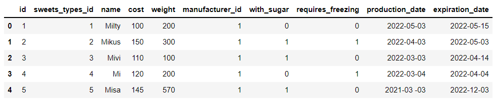
We have built a total of 5 Data sets , It mainly involves desserts 、 Types of desserts and data of processing and storage , For example, the data set of desserts mainly includes the weight of desserts 、 Sugar content 、 Production date and expiration time 、 Cost and other data , as well as :
df_manufacturers = pd.read_sql("SELECT * FROM manufacturers", connector)output
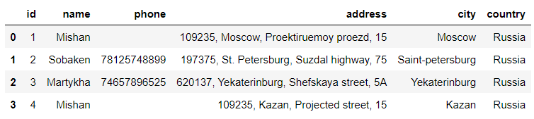
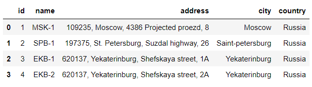
The data set of processing involves the main person in charge and contact information of the factory , The warehouse data set involves the detailed address of the warehouse 、 City location, etc .
df_storehouses = pd.read_sql("SELECT * FROM storehouses", connector)output
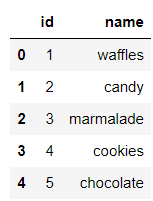
And the dessert category data set ,
df_sweets_types = pd.read_sql("SELECT * FROM sweets_types;", connector)output

Data screening
Screening of simple conditions
Next, let's do some data screening , For example, the weight of desserts is equal to 300 The name of dessert , stay Pandas The code in the module looks like this
# Convert data type
df_sweets['weight'] = pd.to_numeric(df_sweets['weight'])
# Output results
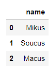
df_sweets[df_sweets.weight == 300].nameoutput
1      Mikus
6     Soucus
11     Macus
Name: name, dtype: object
Of course, we can also pass pandas In the middle of read_sql() Method to call SQL sentence
pd.read_sql("SELECT name FROM sweets WHERE weight = '300'", connector)output
Let's look at a similar case , The screening cost is equal to 100 The name of dessert , The code is as follows
# Pandas
df_sweets['cost'] = pd.to_numeric(df_sweets['cost'])
df_sweets[df_sweets.cost == 100].name

# SQL
pd.read_sql("SELECT name FROM sweets WHERE cost = '100'", connector)
output
MiltyFor text data , We can also further screen out the data we want , The code is as follows
# Pandas
df_sweets[df_sweets.name.str.startswith('M')].name
# SQL
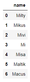
pd.read_sql("SELECT name FROM sweets WHERE name LIKE 'M%'", connector)output
Milty
Mikus
Mivi
Mi
Misa
Maltik
Macus
Of course. SQL Wildcards in statements ,% Means to match any number of letters , and _ Means to match any letter , The specific differences are as follows
# SQL
pd.read_sql("SELECT name FROM sweets WHERE name LIKE 'M%'", connector)
output
pd.read_sql("SELECT name FROM sweets WHERE name LIKE 'M_'", connector)output

Screening of complex conditions
Let's take a look at data filtering with multiple conditions , For example, we want the weight to be equal to 300 And the cost price is controlled at 150 The name of dessert , The code is as follows
# Pandas
df_sweets[(df_sweets.cost == 150) & (df_sweets.weight == 300)].name

# SQL
pd.read_sql("SELECT name FROM sweets WHERE cost = '150' AND weight = '300'", connector)
output
MikusOr the cost price can be controlled within 200-300 Dessert name between , The code is as follows
# Pandas
df_sweets[df_sweets['cost'].between(200, 300)].name

# SQL
pd.read_sql("SELECT name FROM sweets WHERE cost BETWEEN '200' AND '300'", connector)
output

If it comes to sorting , stay SQL It uses ORDER BY sentence , The code is as follows
# SQL
pd.read_sql("SELECT name FROM sweets ORDER BY id DESC", connector)
output
And in the Pandas What is called in the module is sort_values() Method , The code is as follows
# Pandas
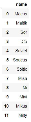
df_sweets.sort_values(by='id', ascending=False).nameoutput
11     Macus
10    Maltik
9        Sor
8         Co
7     Soviet
6     Soucus
5     Soltic
4       Misa
3         Mi
2       Mivi
1      Mikus
0      Milty
Name: name, dtype: object
Select the dessert name with the highest cost price , stay Pandas The code in the module looks like this
df_sweets[df_sweets.cost == df_sweets.cost.max()].nameoutput
11    Macus
Name: name, dtype: object
And in the SQL The code in the statement , We need to first screen out which dessert is the most expensive , Then proceed with further processing , The code is as follows
pd.read_sql("SELECT name FROM sweets WHERE cost = (SELECT MAX(cost) FROM sweets)", connector) We want to see which cities are warehousing , stay Pandas The code in the module looks like this , By calling unique() Method
df_storehouses['city'].unique()output
array(['Moscow', 'Saint-petersburg', 'Yekaterinburg'], dtype=object) And in the SQL The corresponding sentence is DISTINCT keyword
pd.read_sql("SELECT DISTINCT city FROM storehouses", connector)
Data grouping Statistics
stay Pandas Group statistics in modules generally call groupby() Method , Then add a statistical function later , For example, it is to calculate the mean value of scores mean() Method , Or summative sum() Methods, etc. , For example, we want to find out the names of desserts produced and processed in more than one city , The code is as follows
df_manufacturers.groupby('name').name.count()[df_manufacturers.groupby('name').name.count() > 1]output
name
Mishan    2
Name: name, dtype: int64
And in the SQL The grouping in the statement is also GROUP BY, If there are other conditions later , It's using HAVING keyword , The code is as follows
pd.read_sql("""
SELECT name, COUNT(name) as 'name_count' FROM manufacturers
GROUP BY name HAVING COUNT(name) > 1
""", connector)
Data merging
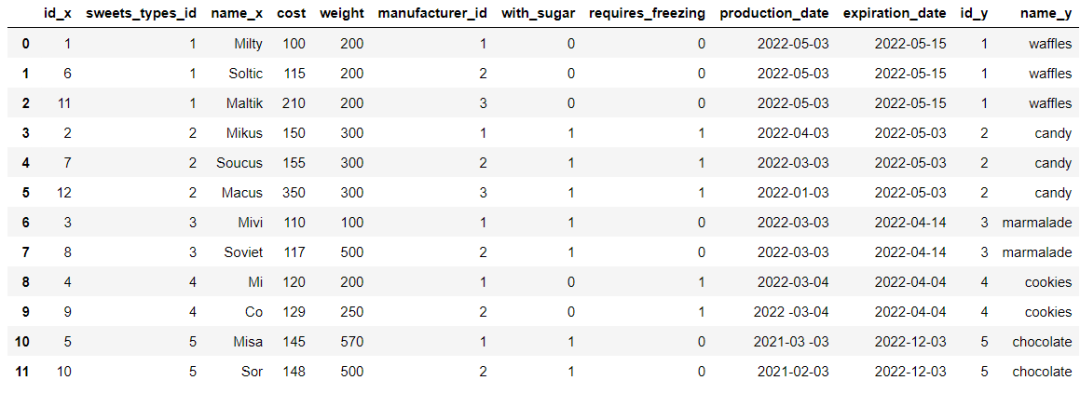
When two or more datasets need to be merged , stay Pandas Modules , We can call merge() Method , For example, we will df_sweets Data set and df_sweets_types Merge the two data sets , among df_sweets In the middle of sweets_types_id Is the foreign key of the table
df_sweets.head()output
df_sweets_types.head()output
The specific data consolidation code is as follows
df_sweets_1 = df_sweets.merge(df_sweets_types, left_on='sweets_types_id', right_on='id')output
We will further screen out chocolate flavored desserts , The code is as follows
df_sweets_1.query('name_y == "chocolate"').name_xoutput
10    Misa
11     Sor
Name: name_x, dtype: object
and SQL The sentence is relatively simple , The code is as follows
# SQL
pd.read_sql("""
SELECT sweets.name FROM sweets
JOIN sweets_types ON sweets.sweets_types_id = sweets_types.id
WHERE sweets_types.name = 'chocolate';
""", connector)
output


The structure of the data set
Let's take a look at the structure of the data set , stay Pandas View directly in the module shape Attribute is enough , The code is as follows
df_sweets.shapeoutput
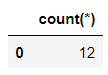
(12, 10) And in the SQL In the sentence , It is
pd.read_sql("SELECT count(*) FROM sweets;", connector)output

Looking back
It's too voluminous !AI High accuracy of math exam 81%
Python Common encryption algorithms in crawlers !
2D Transformation 3D, Look at NVIDIA's AI“ new ” magic !
How to use Python Realize the security system of the scenic spot ?
 Share
 Point collection
 A little bit of praise
Click to see 边栏推荐
- Inftnews | drink tea and send virtual stocks? Analysis of Naixue's tea "coin issuance"
- 基于Cortex-M3、M4的GPIO口位带操作宏定义(可总线输入输出,可用于STM32、ADuCM4050等)
- Vscode configures the typera editor for MD
- Ros2 - workspace (V)
- 使用paping工具进行tcp端口连通性检测
- U-boot initialization and workflow analysis
- 【无标题】
- kata container
- 乐鑫面试流程
- Written examination notes
猜你喜欢

Pycahrm reports an error: indentation error: unindent does not match any outer indentation

Volcano 资源预留特性
Orin 两种刷机方式

Ros2 - first acquaintance with ros2 (I)
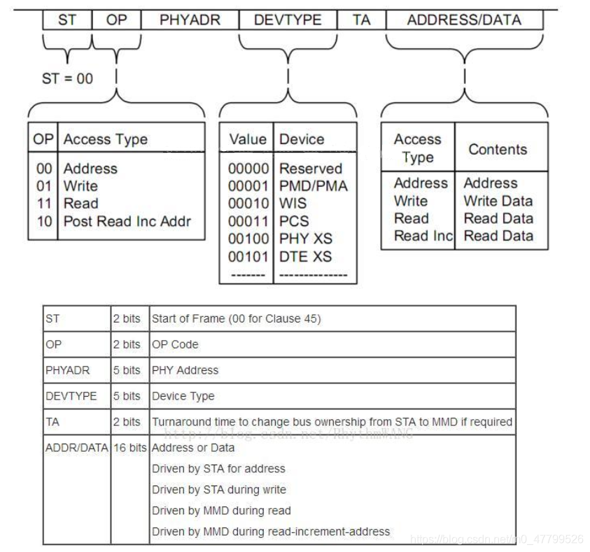
PHY驱动调试之 --- MDIO/MDC接口22号和45号条款(一)
Orin installs CUDA environment

namespace
Orin 安装CUDA环境
PHY drive commissioning --- mdio/mdc interface Clause 22 and 45 (I)
Ros2 - common command line (IV)
随机推荐
Special training of C language array
Interpretation of the earliest sketches - image translation work sketchygan
数学分析_笔记_第8章:重积分
Preemption of CFS scheduling
Xavier CPU & GPU high load power consumption test
Volcano 资源预留特性
Use ffmpeg to rotate, flip up and down, and flip horizontally
What is linting
IPage能正常显示数据,但是total一直等于0
Mipi interface, DVP interface and CSI interface of camera
6-3 find the table length of the linked table
Steps and FAQs of connecting windows Navicat to Alibaba cloud server MySQL
ethtool 原理介绍和解决网卡丢包排查思路(附ethtool源码下载)
C语言数组专题训练
Cookie、Session、JWT、token四者间的区别与联系
kata container
namespace
MySQL setting trigger problem
The problem of Chinese garbled code in the vscode output box can be solved once for life
摄像头的MIPI接口、DVP接口和CSI接口