当前位置:网站首页>Natural language processing series (I) -- RNN Foundation
Natural language processing series (I) -- RNN Foundation
2022-07-02 12:01:00 【raelum】
notes : This article is a concluding article , The narration is relatively simple , Not for beginners
Catalog
One 、 Why would there be RNN?
ordinary MLP Unable to process sequence information ( Text 、 Voice etc. ), This is because the sequence is Indefinite length Of , and MLP The number of neurons in the input layer is fixed .
Two 、RNN Structure
Ordinary MLP Structure ( Take a single hidden layer as an example ):
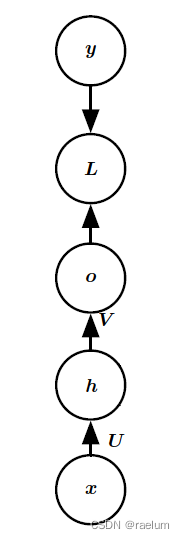
Ordinary RNN( also called Vanilla RNN, This statement will be used next ) Structure ( In single hidden layer MLP On the basis of ):

namely t t t The input received by the time hiding layer comes from t − 1 t-1 t−1 Always hide the output of the layer and t t t Sample input of time . Expressed by mathematical formula , Namely
h ( t ) = tanh ( W h ( t − 1 ) + U x ( t ) + b ) , o ( t ) = V h ( t ) + c , y ^ ( t ) = softmax ( o ( t ) ) h^{(t)}=\tanh(Wh^{(t-1)}+Ux^{(t)}+b),\quad o^{(t)}=Vh^{(t)}+c,\quad \hat{y}^{(t)}=\text{softmax}(o^{(t)}) h(t)=tanh(Wh(t−1)+Ux(t)+b),o(t)=Vh(t)+c,y^(t)=softmax(o(t))
Training RNN In the process of , It's actually learning U , V , W , b , c U,V,W,b,c U,V,W,b,c These parameters .
After positive propagation , We need to calculate the loss , Set a time step t t t The loss obtained at is L ( t ) = L ( t ) ( y ^ ( t ) , y ( t ) ) L^{(t)}=L^{(t)}(\hat{y}^{(t)},y^{(t)}) L(t)=L(t)(y^(t),y(t)), Then the total loss is L = ∑ t = 1 T L ( t ) L=\sum_{t=1}^T L^{(t)} L=∑t=1TL(t).
2.1 BPTT
BPTT(BackPropagation Through Time), Back propagation through time is RNN A term in the training process . Because the forward propagation is along the direction of time passing , And back propagation is carried out against time .
For the convenience of subsequent derivation , Let's improve the symbolic representation first :
h ( t ) = tanh ( W h h h ( t − 1 ) + W x h x ( t ) + b ) , o ( t ) = W h o h ( t ) + c , y ^ ( t ) = softmax ( o ( t ) ) h^{(t)}=\tanh(W_{hh}h^{(t-1)}+W_{xh}x^{(t)}+b),\quad o^{(t)}=W_{ho}h^{(t)}+c,\quad \hat{y}^{(t)}=\text{softmax}(o^{(t)}) h(t)=tanh(Whhh(t−1)+Wxhx(t)+b),o(t)=Whoh(t)+c,y^(t)=softmax(o(t))
Make a horizontal one concatenation: W = ( W h h , W x h ) W=(W_{hh},W_{xh}) W=(Whh,Wxh), For simplicity , Omit offset b b b, Then there are
h ( t ) = tanh ( W ( h ( t − 1 ) x ( t ) ) ) h^{(t)}=\tanh\left(W \begin{pmatrix} h^{(t-1)} \\ x^{(t)} \end{pmatrix} \right) h(t)=tanh(W(h(t−1)x(t)))
, Next we will focus on parameters W W W Learning from .
be aware
∂ h ( t ) ∂ h ( t − 1 ) = tanh ′ ( W h h h ( t − 1 ) + W x h x ( t ) ) W h h , ∂ L ∂ W = ∑ t = 1 T ∂ L ( t ) ∂ W \frac{\partial h^{(t)}}{\partial h^{(t-1)}}=\tanh'(W_{hh}h^{(t-1)}+W_{xh}x^{(t)})W_{hh},\quad \frac{\partial L}{\partial W}=\sum_{t=1}^T\frac{\partial L^{(t)}}{\partial W} ∂h(t−1)∂h(t)=tanh′(Whhh(t−1)+Wxhx(t))Whh,∂W∂L=t=1∑T∂W∂L(t)
thus
∂ L ( T ) ∂ W = ∂ L ( T ) ∂ h ( T ) ⋅ ∂ h ( T ) ∂ h ( T − 1 ) ⋯ ∂ h ( 2 ) ∂ h ( 1 ) ⋅ ∂ h ( 1 ) ∂ W = ∂ L ( T ) ∂ h ( T ) ⋅ ∏ t = 2 T ∂ h ( t ) ∂ h ( t − 1 ) ⋅ ∂ h ( 1 ) ∂ W = ∂ L ( T ) ∂ h ( T ) ⋅ ( ∏ t = 2 T tanh ′ ( W h h h ( t − 1 ) + W x h x ( t ) ) ) ⋅ W h h T − 1 ⋅ ∂ h ( 1 ) ∂ W \begin{aligned} \frac{\partial L^{(T)}}{\partial W}&=\frac{\partial L^{(T)}}{\partial h^{(T)}}\cdot \frac{\partial h^{(T)}}{\partial h^{(T-1)}}\cdots \frac{\partial h^{(2)}}{\partial h^{(1)}}\cdot\frac{\partial h^{(1)}}{\partial W} \\ &=\frac{\partial L^{(T)}}{\partial h^{(T)}}\cdot \prod_{t=2}^T\frac{\partial h^{(t)}}{\partial h^{(t-1)}}\cdot\frac{\partial h^{(1)}}{\partial W}\\ &=\frac{\partial L^{(T)}}{\partial h^{(T)}}\cdot \left(\prod_{t=2}^T\tanh'(W_{hh}h^{(t-1)}+W_{xh}x^{(t)})\right)\cdot W_{hh}^{T-1} \cdot\frac{\partial h^{(1)}}{\partial W}\\ \end{aligned} ∂W∂L(T)=∂h(T)∂L(T)⋅∂h(T−1)∂h(T)⋯∂h(1)∂h(2)⋅∂W∂h(1)=∂h(T)∂L(T)⋅t=2∏T∂h(t−1)∂h(t)⋅∂W∂h(1)=∂h(T)∂L(T)⋅(t=2∏Ttanh′(Whhh(t−1)+Wxhx(t)))⋅WhhT−1⋅∂W∂h(1)
because tanh ′ ( ⋅ ) \tanh'(\cdot) tanh′(⋅) Almost always less than 1 1 1 Of , When T T T When it is large enough, the gradient will disappear .
If the nonlinear activation function is not used , For simplicity , Let's set the activation function as an identity map f ( x ) = x f(x)=x f(x)=x, So there is
∂ L ( T ) ∂ W = ∂ L ( T ) ∂ h ( T ) ⋅ W h h T − 1 ⋅ ∂ h ( 1 ) ∂ W \frac{\partial L^{(T)}}{\partial W}=\frac{\partial L^{(T)}}{\partial h^{(T)}}\cdot W_{hh}^{T-1} \cdot\frac{\partial h^{(1)}}{\partial W} ∂W∂L(T)=∂h(T)∂L(T)⋅WhhT−1⋅∂W∂h(1)
- When W h h W_{hh} Whh The maximum singular value of is greater than 1 1 1 when , There will be a gradient explosion .
- When W h h W_{hh} Whh The maximum singular value of is less than 1 1 1 when , The gradient disappears .
3、 ... and 、RNN The classification of
According to the structure of input and output RNN Classify as follows :
- 1 vs N(vec2seq):Image Captioning;
- N vs 1(seq2vec):Sentiment Analysis;
- N vs M(seq2seq):Machine Translation;
- N vs N(seq2seq):Sequence Labeling(POS Tagging)

Be careful 1 vs 1 It's traditional MLP.
If you classify according to the internal structure, you will get :
- RNN、Bi-RNN、…
- LSTM、Bi-LSTM、…
- GRU、Bi-GRU、…
Four 、Vanilla RNN Advantages and disadvantages
advantage :
- It can handle sequences of variable length ;
- Historical information will be considered in the calculation ;
- Weights are shared in time ;
- The model size will not change as the input size increases .
shortcoming :
- Calculation efficiency is low ;
- The gradient will disappear / The explosion ( Later we will know , Gradient clipping can be used to avoid gradient explosion , To avoid the gradient disappearing, you can use other RNN structure , Such as LSTM);
- Unable to process long sequence ( That is, it does not have long memory );
- Unable to take advantage of future input (Bi-RNN To solve ).
5、 ... and 、Bidirectional RNN
A lot of time , What we want to output y ( t ) y^{(t)} y(t) May depend on the entire sequence , Therefore, we need to use two-way RNN(BRNN).BRNN Combined with the movement in time from the beginning of the sequence RNN And moving from the end of the sequence RNN. Two RNN They are independent of each other and do not share weights :
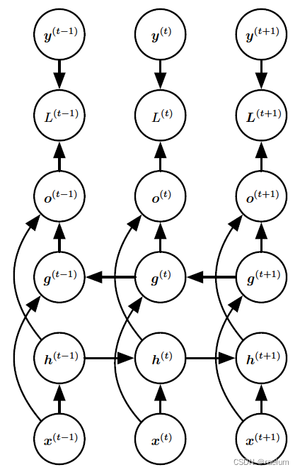
The corresponding calculation method becomes :
h ( t ) = tanh ( W 1 h ( t − 1 ) + U 1 x ( t ) + b 1 ) g ( t ) = tanh ( W 2 h ( t − 1 ) + U 2 x ( t ) + b 2 ) o ( t ) = V ( h ( t ) ; g ( t ) ) + c y ^ ( t ) = softmax ( o ( t ) ) \begin{aligned} &h^{(t)}=\tanh(W_1h^{(t-1)}+U_1x^{(t)}+b_1) \\ &g^{(t)}=\tanh(W_2h^{(t-1)}+U_2x^{(t)}+b_2) \\ &o^{(t)}=V(h^{(t)};g^{(t)})+c \\ &\hat{y}^{(t)}=\text{softmax}(o^{(t)}) \\ \end{aligned} h(t)=tanh(W1h(t−1)+U1x(t)+b1)g(t)=tanh(W2h(t−1)+U2x(t)+b2)o(t)=V(h(t);g(t))+cy^(t)=softmax(o(t))
among ( h ( t ) ; g ( t ) ) (h^{(t)};g^{(t)}) (h(t);g(t)) Represents that the two column vectors h ( t ) h^{(t)} h(t) and g ( t ) g^{(t)} g(t) Make longitudinal connection .
in fact , If the V V V Block by column , Then the third equation above can also be written as :
o ( t ) = V ( h ( t ) ; g ( t ) ) + c = ( V 1 , V 2 ) ( h ( t ) g ( t ) ) + c = V 1 h ( t ) + V 2 g ( t ) + c o^{(t)}=V(h^{(t)};g^{(t)})+c= (V_1,V_2) \begin{pmatrix} h^{(t)} \\ g^{(t)} \end{pmatrix}+c=V_1h^{(t)}+V_2g^{(t)}+c o(t)=V(h(t);g(t))+c=(V1,V2)(h(t)g(t))+c=V1h(t)+V2g(t)+c
Training BRNN The process of learning is actually learning U 1 , U 2 , V , W 1 , W 2 , b 1 , b 2 , c U_1,U_2,V,W_1,W_2,b_1,b_2,c U1,U2,V,W1,W2,b1,b2,c These parameters .
6、 ... and 、Stacked RNN
The stack RNN Also called multilayer RNN Or depth RNN, That is, it is composed of multiple hidden layers . One way with double hidden layers RNN For example , Its structure is as follows :
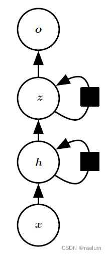
The corresponding calculation process is as follows :
h ( t ) = tanh ( W h h h ( t − 1 ) + W x h x ( t ) + b h ) z ( t ) = tanh ( W z z z ( t − 1 ) + W h z h ( t ) + b z ) o ( t ) = W z o z ( t ) + b o y ^ ( t ) = softmax ( o ( t ) ) \begin{aligned} &h^{(t)}=\tanh(W_{hh}h^{(t-1)}+W_{xh}x^{(t)}+b_h) \\ &z^{(t)}=\tanh(W_{zz}z^{(t-1)}+W_{hz}h^{(t)}+b_z) \\ &o^{(t)}=W_{zo}z^{(t)}+b_o \\ &\hat{y}^{(t)}=\text{softmax}(o^{(t)}) \\ \end{aligned} h(t)=tanh(Whhh(t−1)+Wxhx(t)+bh)z(t)=tanh(Wzzz(t−1)+Whzh(t)+bz)o(t)=Wzoz(t)+boy^(t)=softmax(o(t))
边栏推荐
- PyTorch搭建LSTM实现服装分类(FashionMNIST)
- HOW TO EASILY CREATE BARPLOTS WITH ERROR BARS IN R
- 动态内存(进阶四)
- Orb-slam2 data sharing and transmission between different threads
- Three transparent LED displays that were "crowded" in 2022
- GGPLOT: HOW TO DISPLAY THE LAST VALUE OF EACH LINE AS LABEL
- SVO2系列之深度滤波DepthFilter
- 6方面带你认识LED软膜屏 LED软膜屏尺寸|价格|安装|应用
- QT获取某个日期是第几周
- From scratch, develop a web office suite (3): mouse events
猜你喜欢
HOW TO CREATE AN INTERACTIVE CORRELATION MATRIX HEATMAP IN R
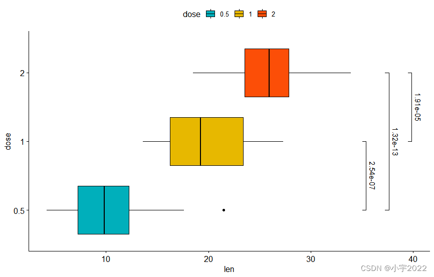
How to Add P-Values onto Horizontal GGPLOTS
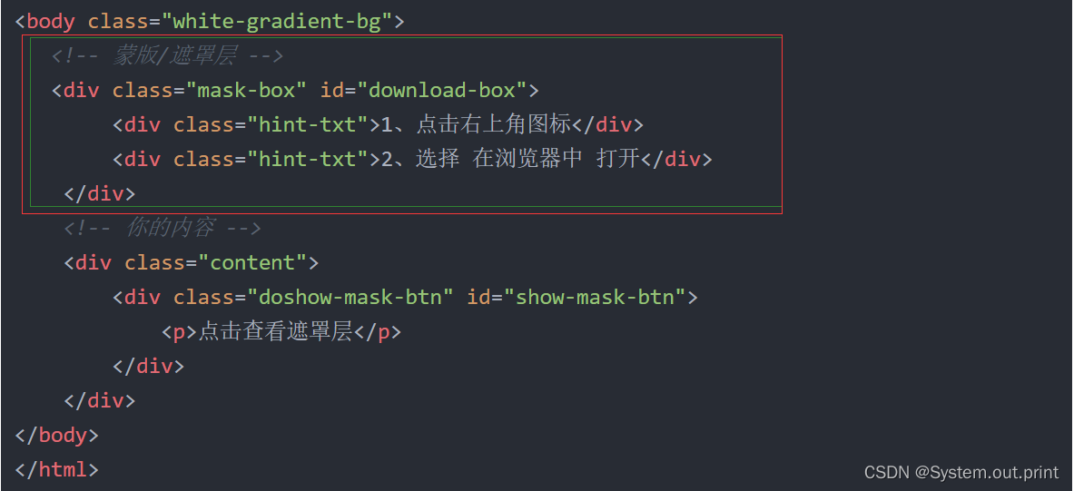
H5, add a mask layer to the page, which is similar to clicking the upper right corner to open it in the browser
How to Add P-Values onto Horizontal GGPLOTS

Beautiful and intelligent, Haval H6 supreme+ makes Yuanxiao travel safer

HOW TO CREATE A BEAUTIFUL INTERACTIVE HEATMAP IN R

GGPlot Examples Best Reference
How to Create a Nice Box and Whisker Plot in R
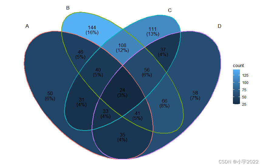
BEAUTIFUL GGPLOT VENN DIAGRAM WITH R
YYGH-BUG-04
随机推荐
ESP32存储配网信息+LED显示配网状态+按键清除配网信息(附源码)
Log4j2
Pyqt5+opencv project practice: microcirculator pictures, video recording and manual comparison software (with source code)
Summary of flutter problems
Log4j2
HOW TO ADD P-VALUES ONTO A GROUPED GGPLOT USING THE GGPUBR R PACKAGE
GGPLOT: HOW TO DISPLAY THE LAST VALUE OF EACH LINE AS LABEL
浅谈sklearn中的数据预处理
自然语言处理系列(三)——LSTM
From scratch, develop a web office suite (3): mouse events
YYGH-BUG-05
YYGH-BUG-04
行业的分析
GGPlot Examples Best Reference
[multithreading] the main thread waits for the sub thread to finish executing, and records the way to execute and obtain the execution result (with annotated code and no pit)
to_bytes与from_bytes简单示例
GGHIGHLIGHT: EASY WAY TO HIGHLIGHT A GGPLOT IN R
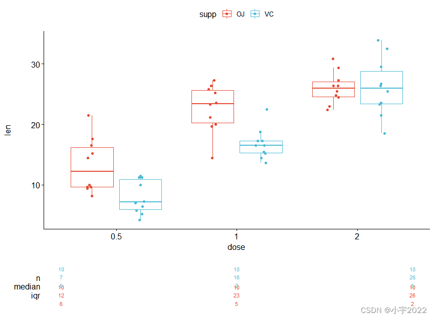
How to Create a Beautiful Plots in R with Summary Statistics Labels
6方面带你认识LED软膜屏 LED软膜屏尺寸|价格|安装|应用
How to Create a Beautiful Plots in R with Summary Statistics Labels