当前位置:网站首页>Market segmentation of supermarket customers based on purchase behavior data (RFM model)
Market segmentation of supermarket customers based on purchase behavior data (RFM model)
2022-07-06 06:39:00 【Nothing (sybh)】
Catalog
subject :
Market segmentation of supermarket customers based on purchase behavior data : Existing supermarket customers' purchasing behavior RFM Data sets ( Data files :RFM data .txt), Please use various clustering algorithms to segment customer groups . Complete the following questions :
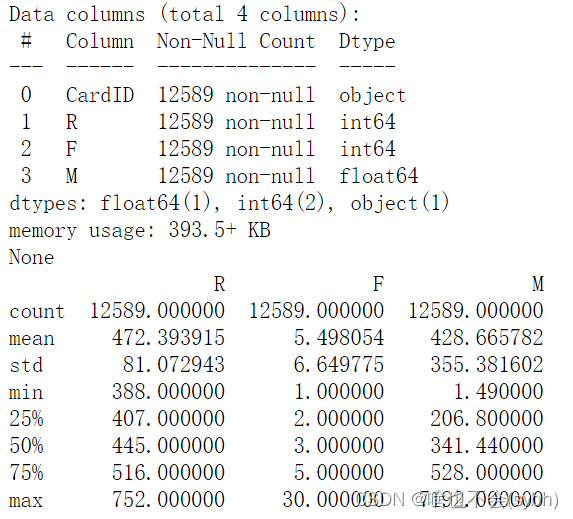
1) Analyze customers' purchasing behavior RFM Data set ,R\F\M What are the distribution characteristics of these three variables ?(10 branch )
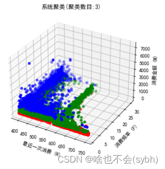
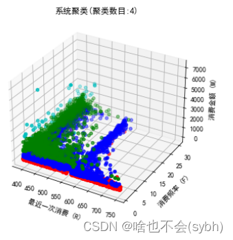
2) Try to divide the purchase into 4 class , And analyze the buying behavior characteristics of each customer .(10 branch )
3) Evaluation model , And analyze and gather 4 Whether the class is appropriate .(30 branch )
One 、 What do you mean RFM?
RFM It is a model for clustering user quality , Corresponding to three indicators
R(Recency): The time interval of the user's last consumption , Measure whether users are likely to lose
F(Frequency)
: The cumulative consumption frequency of users in the recent period , Measure user stickiness
M(Money): The user's accumulated consumption amount in the recent period , Measure users' spending power and loyalty
Two 、 clustering
#  Item 1 : E-commerce user quality RFM Clustering analysis

from sklearn.cluster import KMeans
from sklearn import metrics
import matplotlib.pyplot as plt
from sklearn import preprocessing

#  Import and clean data
data = pd.read_table('RFM data .txt',sep=" ")
# data=pd.read_table("RFM data .txt",encoding="gbk",sep=" ")
# data.user_id = data.user_id.astype('str')
print(data.info())
print(data.describe())
X = data.values[:,1:]

#  Data standardization (z_score)
Model = preprocessing.StandardScaler()
X = Model.fit_transform(X)

#  iteration , Choose the right one K
ch_score = []
ss_score = []
inertia = []
for k in range(2,10):
    clf = KMeans(n_clusters=k,max_iter=1000)
    pred = clf.fit_predict(X)
    ch = metrics.calinski_harabasz_score(X,pred)
    ss = metrics.silhouette_score(X,pred)
    ch_score.append(ch)
    ss_score.append(ss)
    inertia.append(clf.inertia_)

#  Make a comparison
fig = plt.figure()
ax1 = fig.add_subplot(131)
plt.plot(list(range(2,10)),ch_score,label='ch',c='y')
plt.title('CH(calinski_harabaz_score)')
plt.legend()

ax2 = fig.add_subplot(132)
plt.plot(list(range(2,10)),ss_score,label='ss',c='b')
plt.title(' Profile factor ')
plt.legend()

ax3 = fig.add_subplot(133)
plt.plot(list(range(2,10)),inertia,label='inertia',c='g')
plt.title('inertia')
plt.legend()
plt.rcParams['font.sans-serif'] = ['SimHei']
plt.rcParams['font.serif'] = ['SimHei']  #  Set the normal display of Chinese
plt.show()
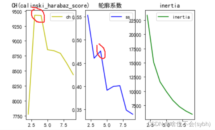
This time, we use 3 The clustering quality is comprehensively determined by three indicators ,CH, Contour coefficient and inertia fraction , The first 1 And the 3 The bigger the better , The contour coefficient is closer to 1 The better , Taken together , Gather into 4 Class effect is better
CH The bigger the indicator , The better the clustering effect is
clf.inertia_ It is a clustering evaluation index , I often use this . Talk about his shortcomings : This evaluation parameter represents the sum of the distances from a certain point in the cluster to the cluster , Although this method shows the fineness of clustering when the evaluation parameters are the smallest , But in this case, the division will be too fine , And it does not consider maximizing the distance from the point outside the cluster , therefore , I recommend method 2 :
Use the contour coefficient method K Choice of value , Here it is , I need to explain the contour coefficient , And why the contour coefficient is selected as the standard of internal evaluation , The formula of contour coefficient is :S=(b-a)/max(a,b), among a Is the average distance between a single sample and all samples in the same cluster ,b Is the average of all samples from a single sample to different clusters .
# According to the best K value , Clustering results
model = KMeans(n_clusters=4,max_iter=1000)
model.fit_predict(X)
labels = pd.Series(model.labels_)
centers = pd.DataFrame(model.cluster_centers_)
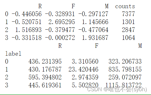
result1 = pd.concat([centers,labels.value_counts().sort_index(ascending=True)],axis=1) # Put the cluster center and the number of clusters together
result1.columns = list(data.columns[1:]) + ['counts']
print(result1)
result = pd.concat([data,labels],axis=1) # Put the original data and clustering results together
result.columns = list(data.columns)+['label'] # Change column names
pd.options.display.max_columns = None # Set to show all columns
print(result.groupby(['label']).agg('mean')) # Calculate the mean value of each index in groups
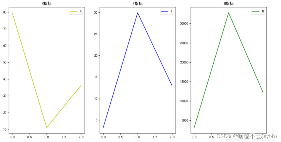
#  Map the clustering results

fig = plt.figure()
ax1= fig.add_subplot(131)
ax1.plot(list(range(1,5)),result1.R,c='y',label='R')
plt.title('R indicators ')
plt.legend()
ax2= fig.add_subplot(132)
ax2.plot(list(range(1,5)),result1.F,c='b',label='F')
plt.title('F indicators ')
plt.legend()
ax3= fig.add_subplot(133)
ax3.plot(list(range(1,5)),result1.M,c='g',label='M')
plt.title('M indicators ')
plt.legend()
plt.show()
3、 ... and 、 Result analysis
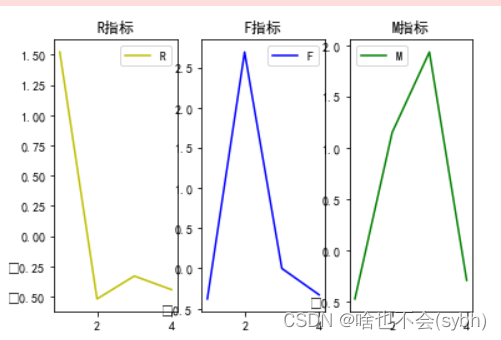
1. Losing customers : Long consumption cycle 、 Less consumption 、 Consumption capacity is almost zero
2. Active customers : The consumption cycle is short 、 More times of consumption 、 Strong consumption ability
3.VIP customer : The consumption cycle is general 、 Consumption times are average 、 Consumption capacity is very strong
4. Wandering customers : The consumption cycle is general 、 Less consumption 、 Average spending power

1. Losing customers : Long consumption cycle 、 Less consumption 、 Consumption capacity is almost zero
2.vip customer : The consumption cycle is short 、 More times of consumption 、 Consumption capacity is very strong
3. Ordinary customers : The consumption cycle is general 、 Consumption times are average 、 Average spending power
边栏推荐
- Drug disease association prediction based on multi-scale heterogeneous network topology information and multiple attributes
- University of Manchester | dda3c: collaborative distributed deep reinforcement learning in swarm agent systems
- 钓鱼&文件名反转&office远程模板
- 记一个基于JEECG-BOOT的比较复杂的增删改功能的实现
- 关于新冠疫情,常用的英文单词、语句有哪些?
- ML之shap:基于adult人口普查收入二分类预测数据集(预测年收入是否超过50k)利用Shap值对XGBoost模型实现可解释性案例之详细攻略
- Mise en œuvre d’une fonction complexe d’ajout, de suppression et de modification basée sur jeecg - boot
- Office-DOC加载宏-上线CS
- [ 英语 ] 语法重塑 之 动词分类 —— 英语兔学习笔记(2)
- 电子书-CHM-上线CS
猜你喜欢
Redis core technology and basic architecture of actual combat: what does a key value database contain?
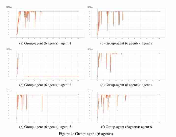
University of Manchester | dda3c: collaborative distributed deep reinforcement learning in swarm agent systems
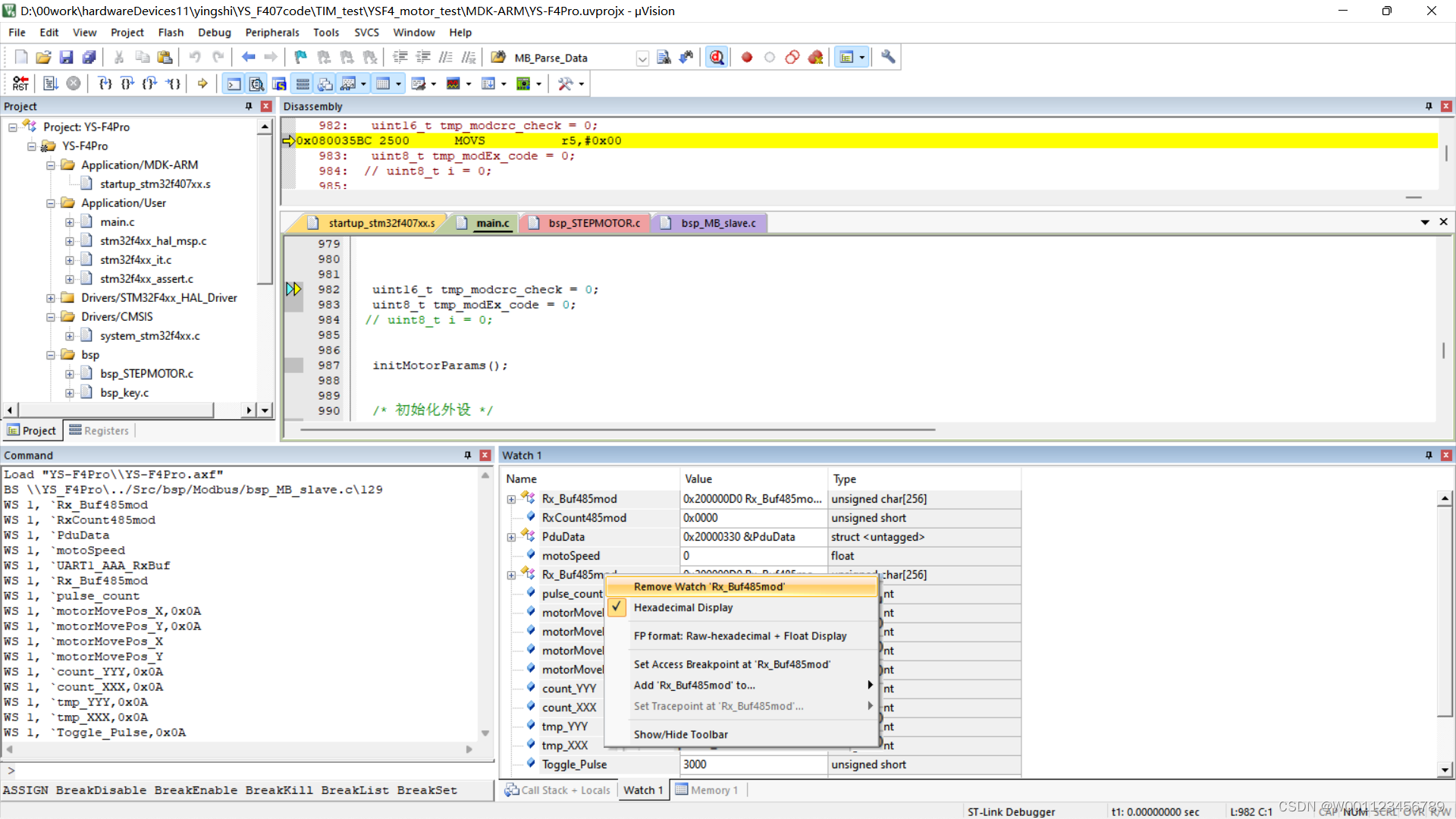
Delete the variables added to watch1 in keil MDK

Chinese English comparison: you can do this Best of luck

翻译公司证件盖章的价格是多少

论文摘要翻译,多语言纯人工翻译

今日夏至 Today‘s summer solstice

国际经贸合同翻译 中译英怎样效果好
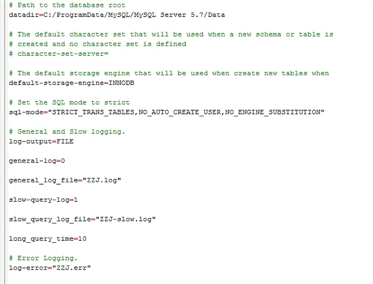
MySQL5.72.msi安装失败

如何做好金融文献翻译?
随机推荐
LeetCode每日一题(1870. Minimum Speed to Arrive on Time)
E-book CHM online CS
How to do a good job in financial literature translation?
Thesis abstract translation, multilingual pure human translation
我的创作纪念日
Luogu p2141 abacus mental arithmetic test
Remember the implementation of a relatively complex addition, deletion and modification function based on jeecg-boot
How do programmers remember code and programming language?
红蓝对抗之流量加密(Openssl加密传输、MSF流量加密、CS修改profile进行流量加密)
Cobalt strike feature modification
QT: the program input point xxxxx cannot be located in the dynamic link library.
MySQL5.72.msi安装失败
Use shortcut LNK online CS
[web security] nodejs prototype chain pollution analysis
LeetCode 1200. Minimum absolute difference
Drug disease association prediction based on multi-scale heterogeneous network topology information and multiple attributes
Suspended else
Traffic encryption of red blue confrontation (OpenSSL encrypted transmission, MSF traffic encryption, CS modifying profile for traffic encryption)
Modify the list page on the basis of jeecg boot code generation (combined with customized components)
MySQL is sorted alphabetically