当前位置:网站首页>[the Nine Yang Manual] 2019 Fudan University Applied Statistics real problem + analysis
[the Nine Yang Manual] 2019 Fudan University Applied Statistics real problem + analysis
2022-07-06 13:30:00 【Elder martial brother statistics】
Catalog
The real part
One 、(15 branch ) There is n − 1 n-1 n−1 A white ball 1 A black ball , There is n n n A white ball , Take one ball from each of the two bags for Exchange , Seek exchange N N N The probability that the black ball will still be in the armour pocket after times .
Two 、(15 branch ) f ( x , y ) = A e − ( 2 x + 3 y ) I [ x > 0 , y > 0 ] , f(x, y)=A e^{-(2 x+3 y)} I[x>0, y>0], f(x,y)=Ae−(2x+3y)I[x>0,y>0], seek
(1)(3 branch ) A A A;
(2)(3 branch ) P ( X < 2 , Y < 1 ) P(X<2, Y<1) P(X<2,Y<1);
(3)(3 branch ) X X X Marginal density of ;
(4)(3 branch ) P ( X < 3 ∣ Y < 1 ) P(X<3 \mid Y<1) P(X<3∣Y<1);
(5)(3 branch ) f ( x ∣ y ) f(x \mid y) f(x∣y).
3、 ... and 、(10 branch ) X 1 , X 2 , X_{1}, X_{2}, X1,X2,i.i.d ∼ N ( μ , σ 2 ) , \sim N\left(\mu, \sigma^{2}\right), ∼N(μ,σ2), seek E max { X 1 , X 2 } E \max \left\{X_{1}, X_{2}\right\} Emax{ X1,X2}.
Four 、(20 branch ) E X = 0 , Var ( X ) = σ 2 , E X=0, \operatorname{Var}(X)=\sigma^{2}, EX=0,Var(X)=σ2, Prove for any ε > 0 , \varepsilon>0, ε>0, Yes
(1)(10 branch ) P ( ∣ X ∣ > ε ) ≤ σ 2 ε 2 P(|X|>\varepsilon) \leq \frac{\sigma^{2}}{\varepsilon^{2}} P(∣X∣>ε)≤ε2σ2;
(2)(10 branch ) P ( X > ε ) ≤ σ 2 σ 2 + ε 2 P(X>\varepsilon) \leq \frac{\sigma^{2}}{\sigma^{2}+\varepsilon^{2}} P(X>ε)≤σ2+ε2σ2.
5、 ... and 、(10 branch ) X 1 , X 2 , i . i . d ∼ N ( 0 , 1 ) , X_{1}, X_{2}, i . i . d \sim N(0,1), X1,X2,i.i.d∼N(0,1), seek X 1 X 2 \frac{X_{1}}{X_{2}} X2X1 The distribution of .
6、 ... and 、(20 branch ) X 1 , X 2 , … , X n , i . i . d ∼ N ( μ , σ 2 ) , μ X_{1}, X_{2}, \ldots, X_{n}, i . i . d \sim N\left(\mu, \sigma^{2}\right), \mu X1,X2,…,Xn,i.i.d∼N(μ,σ2),μ It is known that , prove :
(1)(10 branch ) 1 n ∑ i = 1 n ( X i − μ ) 2 \frac{1}{n} \sum_{i=1}^{n}\left(X_{i}-\mu\right)^{2} n1∑i=1n(Xi−μ)2 yes σ 2 \sigma^{2} σ2 Effective estimation of ;
(2)(10 branch ) 1 n π 2 ∑ i = 1 n ∣ X i − μ ∣ \frac{1}{n} \sqrt{\frac{\pi}{2}} \sum_{i=1}^{n}\left|X_{i}-\mu\right| n12π∑i=1n∣Xi−μ∣ yes σ \sigma σ Unbiased estimation of , But it's not effective .
7、 ... and 、(20 branch ) The overall distribution function F ( x ) F(x) F(x) Continuous single increase , X ( 1 ) , X ( 2 ) , … , X ( n ) X_{(1)}, X_{(2)}, \ldots, X_{(n)} X(1),X(2),…,X(n) Is the order statistic of random samples from the population , Y i = F ( X ( i ) ) , Y_{i}=F\left(X_{(i)}\right), Yi=F(X(i)), seek
(1)(10 branch ) E Y i , Var ( Y i ) E Y_{i}, \operatorname{Var}\left(Y_{i}\right) EYi,Var(Yi);
(2)(10 branch ) ( Y 1 , Y 2 , … , Y n ) T \left(Y_{1}, Y_{2}, \ldots, Y_{n}\right)^{T} (Y1,Y2,…,Yn)T The covariance matrix of .
8、 ... and 、(20 branch ) Some come from the general U ( θ , 2 θ ) U(\theta,2\theta) U(θ,2θ) A random sample of X 1 , ⋯ , X n X_1,\cdots,X_n X1,⋯,Xn, seek θ \theta θ Moment estimation sum of MLE, And verify the unbiasedness and consistency .
Nine 、(20 branch ) set up X 1 , ⋯ , X n X_1,\cdots,X_n X1,⋯,Xn Is from N ( μ , 1 ) N(\mu,1) N(μ,1) A random sample of , Consider the hypothesis test problem H 0 : μ = 1 v s H 1 : μ = 2 H_0:\mu = 1 \quad \mathrm{vs} \quad H_1:\mu=2 H0:μ=1vsH1:μ=2 Given denial domain W = { X ˉ > 1.6 } W=\{\bar{X}>1.6\} W={ Xˉ>1.6}, Answer the following questions :
(1)(10 branch ) Find the probability of making two kinds of mistakes α \alpha α, β \beta β;
(2)(10 branch ) Request the second kind of error β ≤ 0.01 \beta\le0.01 β≤0.01, Find the value range of the sample size .
The analysis part
One 、(15 branch ) There is n − 1 n-1 n−1 A white ball 1 A black ball , There is n n n A white ball , Take one ball from each of the two bags for Exchange , Seek exchange N N N The probability that the black ball will still be in the armour pocket after times .
Solution:
set up p k p_{k} pk For exchange k k k The probability that the black ball will still be in the armour pocket after times , Then according to the full probability formula ,
p k + 1 = p k ⋅ n − 1 n + ( 1 − p k ) ⋅ 1 n = ( 1 − 2 n ) p k + 1 n , p_{k+1}=p_{k} \cdot \frac{n-1}{n}+\left(1-p_{k}\right) \cdot \frac{1}{n}=\left(1-\frac{2}{n}\right) p_{k}+\frac{1}{n}, pk+1=pk⋅nn−1+(1−pk)⋅n1=(1−n2)pk+n1, There are p N − 1 2 = ( 1 − 2 n ) ( p N − 1 − 1 2 ) = ⋯ = ( 1 − 2 n ) N ( p 0 − 1 2 ) , p_{N}-\frac{1}{2}=\left(1-\frac{2}{n}\right)\left(p_{N-1}-\frac{1}{2}\right)=\cdots=\left(1-\frac{2}{n}\right)^{N}\left(p_{0}-\frac{1}{2}\right), pN−21=(1−n2)(pN−1−21)=⋯=(1−n2)N(p0−21), namely p N = 1 2 + 1 2 ( 1 − 2 n ) N . p_{N}=\frac{1}{2}+\frac{1}{2}\left(1-\frac{2}{n}\right)^{N} \text {. } pN=21+21(1−n2)N.
Two 、(15 branch ) f ( x , y ) = A e − ( 2 x + 3 y ) I [ x > 0 , y > 0 ] , f(x, y)=A e^{-(2 x+3 y)} I[x>0, y>0], f(x,y)=Ae−(2x+3y)I[x>0,y>0], seek
(1)(3 branch ) A A A;
(2)(3 branch ) P ( X < 2 , Y < 1 ) P(X<2, Y<1) P(X<2,Y<1);
(3)(3 branch ) X X X Marginal density of ;
(4)(3 branch ) P ( X < 3 ∣ Y < 1 ) P(X<3 \mid Y<1) P(X<3∣Y<1);
(5)(3 branch ) f ( x ∣ y ) f(x \mid y) f(x∣y).
Solution:
(1) By the regularity of probability , 1 = ∫ R 2 f ( x , y ) d x d y = A ∫ 0 + ∞ e − 2 x d x ∫ 0 + ∞ e − 3 y d y = A 6 ⇒ A = 6 1=\int_{R^{2}} f(x, y) d x d y=A \int_{0}^{+\infty} e^{-2 x} d x \int_{0}^{+\infty} e^{-3 y} d y=\frac{A}{6} \Rightarrow A=6 1=∫R2f(x,y)dxdy=A∫0+∞e−2xdx∫0+∞e−3ydy=6A⇒A=6.
(2) P ( X < 2 , Y < 1 ) = 6 ∫ 0 2 e − 2 x d x ∫ 0 1 e − 3 y d y = 6 ( 1 − e − 4 ) ( 1 − e − 3 ) P(X<2, Y<1)=6 \int_{0}^{2} e^{-2 x} d x \int_{0}^{1} e^{-3 y} d y=6\left(1-e^{-4}\right)\left(1-e^{-3}\right) P(X<2,Y<1)=6∫02e−2xdx∫01e−3ydy=6(1−e−4)(1−e−3).
(3) f X ( x ) = ∫ 0 + ∞ 6 e − 2 x − 3 y d y = 2 e − 2 x , x > 0 f_{X}(x)=\int_{0}^{+\infty} 6 e^{-2 x-3 y} d y=2 e^{-2 x}, x>0 fX(x)=∫0+∞6e−2x−3ydy=2e−2x,x>0.
(4) because f X ( x ) = 2 e − 2 x , f Y ( y ) = 3 e − 3 y f_{X}(x)=2 e^{-2 x}, f_{Y}(y)=3 e^{-3 y} fX(x)=2e−2x,fY(y)=3e−3y, so X , Y X, Y X,Y Are independent of each other , therefore P ( X < 3 ∣ Y < 1 ) = P ( X < 3 ) = 1 − e − 6 . P(X<3 \mid Y<1)=P(X<3)=1-e^{-6} . P(X<3∣Y<1)=P(X<3)=1−e−6.(5) f ( x ∣ y ) = f ( x , y ) f Y ( y ) = 2 e − 2 x , x > 0 , y > 0 f(x \mid y)=\frac{f(x, y)}{f_{Y}(y)}=2 e^{-2 x}, x>0, y>0 f(x∣y)=fY(y)f(x,y)=2e−2x,x>0,y>0.
3、 ... and 、(10 branch ) X 1 , X 2 , X_{1}, X_{2}, X1,X2,i.i.d ∼ N ( μ , σ 2 ) , \sim N\left(\mu, \sigma^{2}\right), ∼N(μ,σ2), seek E max { X 1 , X 2 } E \max \left\{X_{1}, X_{2}\right\} Emax{ X1,X2}.
Solution:
Make Y i = X i − μ σ , i = 1 , 2 Y_{i}=\frac{X_{i}-\mu}{\sigma}, i=1,2 Yi=σXi−μ,i=1,2, so max { Y 1 , Y 2 } = max { X 1 , X 2 } − μ σ \max \left\{Y_{1}, Y_{2}\right\}=\frac{\max \left\{X_{1}, X_{2}\right\}-\mu}{\sigma} max{ Y1,Y2}=σmax{ X1,X2}−μ.
and E max { Y 1 , Y 2 } = E Y 1 I [ Y 1 ≥ Y 2 ] + E Y 2 I [ Y 1 < Y 2 ] = 2 E Y 1 I [ Y 1 ≥ Y 2 ] , E \max \left\{Y_{1}, Y_{2}\right\}=E Y_{1} I_{\left[Y_{1} \geq Y_{2}\right]}+E Y_{2} I_{\left[Y_{1}<Y_{2}\right]}=2 E Y_{1} I_{\left[Y_{1} \geq Y_{2}\right]}, Emax{ Y1,Y2}=EY1I[Y1≥Y2]+EY2I[Y1<Y2]=2EY1I[Y1≥Y2], E [ Y 1 I [ Y 1 ≥ Y 2 ] ] = 1 2 π ∫ − ∞ + ∞ ∫ x + ∞ y e − x 2 + y 2 2 d x d y = 1 2 π ∫ π 4 5 π 4 sin θ d θ ∫ 0 + ∞ r 2 e − r 2 2 d r E[ Y_{1} I_{\left[Y_{1} \geq Y_{2}\right]}]=\frac{1}{2 \pi} \int_{-\infty}^{+\infty} \int_{x}^{+\infty} y e^{-\frac{x^{2}+y^{2}}{2}} d x d y=\frac{1}{2 \pi} \int_{\frac{\pi}{4}}^{\frac{5 \pi}{4}} \sin \theta d \theta \int_{0}^{+\infty} r^{2} e^{-\frac{r^{2}}{2}} d r E[Y1I[Y1≥Y2]]=2π1∫−∞+∞∫x+∞ye−2x2+y2dxdy=2π1∫4π45πsinθdθ∫0+∞r2e−2r2dr
among ∫ 0 + ∞ r 2 e − r 2 2 d r = 2 ∫ 0 + ∞ r 2 2 e − r 2 2 d ( r 2 2 ) = 2 Γ ( 3 2 ) = π 2 \int_{0}^{+\infty} r^{2} e^{-\frac{r^{2}}{2}} d r=\sqrt{2} \int_{0}^{+\infty} \sqrt{\frac{r^{2}}{2}} e^{-\frac{r^{2}}{2}} d\left(\frac{r^{2}}{2}\right)=\sqrt{2} \Gamma\left(\frac{3}{2}\right)=\sqrt{\frac{\pi}{2}} ∫0+∞r2e−2r2dr=2∫0+∞2r2e−2r2d(2r2)=2Γ(23)=2π, so E max { Y 1 , Y 2 } = 1 π , E max { X 1 , X 2 } = μ + σ π E \max \left\{Y_{1}, Y_{2}\right\}=\frac{1}{\sqrt{\pi}}, E \max \left\{X_{1}, X_{2}\right\}=\mu+\frac{\sigma}{\sqrt{\pi}} Emax{ Y1,Y2}=π1,Emax{ X1,X2}=μ+πσ.
Four 、(20 branch ) E X = 0 , Var ( X ) = σ 2 , E X=0, \operatorname{Var}(X)=\sigma^{2}, EX=0,Var(X)=σ2, Prove for any ε > 0 , \varepsilon>0, ε>0, Yes
(1)(10 branch ) P ( ∣ X ∣ > ε ) ≤ σ 2 ε 2 P(|X|>\varepsilon) \leq \frac{\sigma^{2}}{\varepsilon^{2}} P(∣X∣>ε)≤ε2σ2;
(2)(10 branch ) P ( X > ε ) ≤ σ 2 σ 2 + ε 2 P(X>\varepsilon) \leq \frac{\sigma^{2}}{\sigma^{2}+\varepsilon^{2}} P(X>ε)≤σ2+ε2σ2.
Solution:
(1) remember I [ ∣ X ∣ > ε ] = { 1 , ∣ X ∣ > ε , 0 , ∣ X ∣ ≤ ε . I_{[|X|>\varepsilon]}=\left\{\begin{array}{ll}1, & |X|>\varepsilon, \\ 0, & |X| \leq \varepsilon .\end{array}\right. I[∣X∣>ε]={ 1,0,∣X∣>ε,∣X∣≤ε. It's a collection { ω : ∣ X ( ω ) ∣ > ε } \{\omega:|X(\omega)|>\varepsilon\} { ω:∣X(ω)∣>ε} The indicative function of , It can be seen that : I [ ∣ X ∣ > ε ] ≤ ∣ X ∣ 2 ε 2 I_{[|X|>\varepsilon]} \leq \frac{|X|^{2}}{\varepsilon^{2}} I[∣X∣>ε]≤ε2∣X∣2 so P ( ∣ X ∣ > ε ) = E I [ ∣ X ∣ > ε ] ≤ E ∣ X ∣ 2 ε 2 = σ 2 ε 2 P(|X|>\varepsilon)=E I_{[|X|>\varepsilon]} \leq \frac{E|X|^{2}}{\varepsilon^{2}}=\frac{\sigma^{2}}{\varepsilon^{2}} P(∣X∣>ε)=EI[∣X∣>ε]≤ε2E∣X∣2=ε2σ2.
(2) By Markov inequality , Yes P ( X > ε ) = P ( X + a > ε + a ) ≤ E ( X + a ) 2 ( ε + a ) 2 = σ 2 + a 2 ( ε + a ) 2 , P(X>\varepsilon)=P(X+a>\varepsilon+a) \leq \frac{E(X+a)^{2}}{(\varepsilon+a)^{2}}=\frac{\sigma^{2}+a^{2}}{(\varepsilon+a)^{2}}, P(X>ε)=P(X+a>ε+a)≤(ε+a)2E(X+a)2=(ε+a)2σ2+a2, take a = σ 2 ε a=\frac{\sigma^{2}}{\varepsilon} a=εσ2, Then there happens to be σ 2 + a 2 ( ε + a ) 2 = σ 2 + σ 4 ε 2 ( ε + σ 2 ε ) 2 = σ 2 σ 2 + ε 2 , \frac{\sigma^{2}+a^{2}}{(\varepsilon+a)^{2}}=\frac{\sigma^{2}+\frac{\sigma^{4}}{\varepsilon^{2}}}{\left(\varepsilon+\frac{\sigma^{2}}{\varepsilon}\right)^{2}}=\frac{\sigma^{2}}{\sigma^{2}+\varepsilon^{2}}, (ε+a)2σ2+a2=(ε+εσ2)2σ2+ε2σ4=σ2+ε2σ2, therefore P ( X > ε ) ≤ σ 2 σ 2 + ε 2 P(X>\varepsilon) \leq \frac{\sigma^{2}}{\sigma^{2}+\varepsilon^{2}} P(X>ε)≤σ2+ε2σ2.
5、 ... and 、(10 branch ) X 1 , X 2 X_{1}, X_{2} X1,X2, i.i.d. ∼ N ( 0 , 1 ) , \sim N(0,1), ∼N(0,1), seek X 1 X 2 \frac{X_{1}}{X_{2}} X2X1 The distribution of .
Solution:
Due to denominator X 2 X_{2} X2 The distribution of is about 0 symmetry , therefore X 1 ∣ X 2 ∣ \frac{X_{1}}{\left|X_{2}\right|} ∣X2∣X1 And X 1 X 2 \frac{X_{1}}{X_{2}} X2X1 Homodistribution , And obviously N ( 0 , 1 ) χ 2 ( 1 ) 1 \frac{N(0,1)}{\sqrt{\frac{\chi^{2}(1)}{1}}} 1χ2(1)N(0,1) It's a The degree of freedom is 1 Of t t t Distribution , therefore X 1 ∣ X 2 ∣ \frac{X_{1}}{\left|X_{2}\right|} ∣X2∣X1 Also, the degree of freedom is 1 Of t t t Distribution , Its probability density is f ( x ) = Γ ( 1 ) π Γ ( 1 2 ) ( x 2 + 1 ) − 1 = 1 π ⋅ 1 1 + x 2 , − ∞ < x < + ∞ , f(x)=\frac{\Gamma(1)}{\sqrt{\pi} \Gamma\left(\frac{1}{2}\right)}\left(x^{2}+1\right)^{-1}=\frac{1}{\pi} \cdot \frac{1}{1+x^{2}},-\infty<x<+\infty, f(x)=πΓ(21)Γ(1)(x2+1)−1=π1⋅1+x21,−∞<x<+∞, The standard Cauchy distribution .
6、 ... and 、(20 branch ) X 1 , X 2 , … , X n , i . i . d ∼ N ( μ , σ 2 ) , μ X_{1}, X_{2}, \ldots, X_{n}, i . i . d \sim N\left(\mu, \sigma^{2}\right), \mu X1,X2,…,Xn,i.i.d∼N(μ,σ2),μ It is known that , prove :
(1)(10 branch ) 1 n ∑ i = 1 n ( X i − μ ) 2 \frac{1}{n} \sum_{i=1}^{n}\left(X_{i}-\mu\right)^{2} n1∑i=1n(Xi−μ)2 yes σ 2 \sigma^{2} σ2 Effective estimation of ;
(2)(10 branch ) 1 n π 2 ∑ i = 1 n ∣ X i − μ ∣ \frac{1}{n} \sqrt{\frac{\pi}{2}} \sum_{i=1}^{n}\left|X_{i}-\mu\right| n12π∑i=1n∣Xi−μ∣ yes σ \sigma σ Unbiased estimation of , But it's not effective .
Solution:
(1) To calculate σ 2 \sigma^{2} σ2 Of Fisher The amount of information , According to the definition I ( σ 2 ) = E [ ∂ ln f ( X ; σ 2 ) ∂ σ 2 ] 2 = 1 4 σ 4 E [ ( X − μ σ ) 2 − 1 ] 2 , I\left(\sigma^{2}\right)=E\left[\frac{\partial \ln f\left(X ; \sigma^{2}\right)}{\partial \sigma^{2}}\right]^{2}=\frac{1}{4 \sigma^{4}} E\left[\left(\frac{X-\mu}{\sigma}\right)^{2}-1\right]^{2}, I(σ2)=E[∂σ2∂lnf(X;σ2)]2=4σ41E[(σX−μ)2−1]2, just E [ ( X − μ σ ) 2 − 1 ] 2 E\left[\left(\frac{X-\mu}{\sigma}\right)^{2}-1\right]^{2} E[(σX−μ)2−1]2 yes χ 2 \chi^{2} χ2 (1) The variance of , so I ( σ 2 ) = 1 2 σ 4 I\left(\sigma^{2}\right)=\frac{1}{2 \sigma^{4}} I(σ2)=2σ41. therefore , σ 2 \sigma^{2} σ2 Of C-R The lower bound is 1 n I ( σ 2 ) = 2 n σ 4 . \frac{1}{n I\left(\sigma^{2}\right)}=\frac{2}{n} \sigma^{4} . nI(σ2)1=n2σ4. Calculate again 1 n ∑ i = 1 n ( X i − μ ) 2 \frac{1}{n} \sum_{i=1}^{n}\left(X_{i}-\mu\right)^{2} n1∑i=1n(Xi−μ)2 The expected variance of , because 1 σ 2 ∑ i = 1 n ( X i − μ ) 2 ∼ χ 2 ( n ) \frac{1}{\sigma^{2}} \sum_{i=1}^{n}\left(X_{i}-\mu\right)^{2} \sim \chi^{2}(n) σ21∑i=1n(Xi−μ)2∼χ2(n), Expectation is n n n, The variance is 2 n 2 n 2n, therefore E [ 1 n ∑ i = 1 n ( X i − μ ) 2 ] = σ 2 , Var [ 1 n ∑ i = 1 n ( X i − μ ) 2 ] = 2 n σ 4 , E\left[\frac{1}{n} \sum_{i=1}^{n}\left(X_{i}-\mu\right)^{2}\right]=\sigma^{2}, \quad \operatorname{Var}\left[\frac{1}{n} \sum_{i=1}^{n}\left(X_{i}-\mu\right)^{2}\right]=\frac{2}{n} \sigma^{4}, E[n1i=1∑n(Xi−μ)2]=σ2,Var[n1i=1∑n(Xi−μ)2]=n2σ4, It is an unbiased estimate , The variance just reaches C-R Lower bound , Therefore, it is an effective estimate .
(2) First , Make g ( x ) = x g(x)=\sqrt{x} g(x)=x, be σ \sigma σ Of C − R \mathrm{C}-\mathrm{R} C−R The lower bound is [ g ′ ( σ 2 ) ] 2 n I ( σ 2 ) = 1 2 n σ 2 \frac{\left[g^{\prime}\left(\sigma^{2}\right)\right]^{2}}{n I\left(\sigma^{2}\right)}=\frac{1}{2 n} \sigma^{2} nI(σ2)[g′(σ2)]2=2n1σ2, Let's calculate 1 n π 2 ∑ i = 1 n ∣ X i − μ ∣ \frac{1}{n} \sqrt{\frac{\pi}{2}} \sum_{i=1}^{n}\left|X_{i}-\mu\right| n12π∑i=1n∣Xi−μ∣ The expected variance of : 1 σ E ∣ X 1 − μ ∣ = ∫ − ∞ + ∞ ∣ x ∣ 1 2 π e − x 2 2 d x = 2 π ∫ 0 + ∞ x e − x 2 2 d x = 2 π ⇒ E ∣ X 1 − μ ∣ = 2 π σ , \frac{1}{\sigma} E\left|X_{1}-\mu\right|=\int_{-\infty}^{+\infty}|x| \frac{1}{\sqrt{2 \pi}} e^{-\frac{x^{2}}{2}} d x=\sqrt{\frac{2}{\pi}} \int_{0}^{+\infty} x e^{-\frac{x^{2}}{2}} d x=\sqrt{\frac{2}{\pi}} \Rightarrow E\left|X_{1}-\mu\right|=\sqrt{\frac{2}{\pi}} \sigma, σ1E∣X1−μ∣=∫−∞+∞∣x∣2π1e−2x2dx=π2∫0+∞xe−2x2dx=π2⇒E∣X1−μ∣=π2σ, E ∣ X 1 − μ ∣ 2 = σ 2 , so Var ( ∣ X 1 − μ ∣ ) = σ 2 − 2 π σ 2 = ( 1 − 2 π ) σ 2 , E\left|X_{1}-\mu\right|^{2}=\sigma^{2} \text {, so } \operatorname{Var}\left(\left|X_{1}-\mu\right|\right)=\sigma^{2}-\frac{2}{\pi} \sigma^{2}=\left(1-\frac{2}{\pi}\right) \sigma^{2} \text {, } E∣X1−μ∣2=σ2, so Var(∣X1−μ∣)=σ2−π2σ2=(1−π2)σ2, so E [ 1 n π 2 ∑ i = 1 n ∣ X i − μ ∣ ] = σ , Var [ 1 n π 2 ∑ i = 1 n ∣ X i − μ ∣ ] = ( π 2 − 1 ) n σ 2 E\left[\frac{1}{n} \sqrt{\frac{\pi}{2}} \sum_{i=1}^{n}\left|X_{i}-\mu\right|\right]=\sigma, \operatorname{Var}\left[\frac{1}{n} \sqrt{\frac{\pi}{2}} \sum_{i=1}^{n}\left|X_{i}-\mu\right|\right]=\frac{\left(\frac{\pi}{2}-1\right)}{n} \sigma^{2} E[n12π∑i=1n∣Xi−μ∣]=σ,Var[n12π∑i=1n∣Xi−μ∣]=n(2π−1)σ2, It is an unbiased estimate , but Don't reach C-R Lower bound , Not a valid estimate .
7、 ... and 、(20 branch ) The overall distribution function F ( x ) F(x) F(x) Continuous single increase , X ( 1 ) , X ( 2 ) , … , X ( n ) X_{(1)}, X_{(2)}, \ldots, X_{(n)} X(1),X(2),…,X(n) Is the order statistic of random samples from the population , Y i = F ( X ( i ) ) , Y_{i}=F\left(X_{(i)}\right), Yi=F(X(i)), seek
(1)(10 branch ) E Y i , Var ( Y i ) E Y_{i}, \operatorname{Var}\left(Y_{i}\right) EYi,Var(Yi);
(2)(10 branch ) ( Y 1 , Y 2 , … , Y n ) T \left(Y_{1}, Y_{2}, \ldots, Y_{n}\right)^{T} (Y1,Y2,…,Yn)T The covariance matrix of .
Solution:
(1) because U 1 = F ( X 1 ) , U 2 = F ( X 2 ) , ⋯ , U n = F ( X n ) U_{1}=F\left(X_{1}\right), U_{2}=F\left(X_{2}\right), \cdots, U_{n}=F\left(X_{n}\right) U1=F(X1),U2=F(X2),⋯,Un=F(Xn) Independence and obedience [ 0 , 1 ] [0,1] [0,1] Evenly distributed , so Y i = U ( i ) Y_{i}=U_{(i)} Yi=U(i) It happens to be the order statistics of uniform distribution , According to the definition of order statistics , Yes :
f i ( y ) = n ! ( i − 1 ) ! ( n − i ) ! f U ( y ) P i − 1 { U ≤ y } P n − i { U ≥ y } , Insert one by one , Yes f i ( y ) = n ! ( i − 1 ) ! ( n − i ) ! y i − 1 ( 1 − y ) n − i , 0 ≤ y ≤ 1 , Exactly Beta ( i , n − i + 1 ) . \begin{gathered} f_{i}(y)=\frac{n !}{(i-1) !(n-i) !} f_{U}(y) P^{i-1}\{U \leq y\} P^{n-i}\{U \geq y\}, \text { Insert one by one , Yes } \\ f_{i}(y)=\frac{n !}{(i-1) !(n-i) !} y^{i-1}(1-y)^{n-i}, 0 \leq y \leq 1 \text {, Exactly } \operatorname{Beta}(i, n-i+1) . \end{gathered} fi(y)=(i−1)!(n−i)!n!fU(y)Pi−1{ U≤y}Pn−i{ U≥y}, Insert one by one , Yes fi(y)=(i−1)!(n−i)!n!yi−1(1−y)n−i,0≤y≤1, Exactly Beta(i,n−i+1). According to the nature of beta distribution E Y i = i n + 1 , Var ( Y i ) = i ( n − i + 1 ) ( n + 1 ) 2 ( n + 2 ) E Y_{i}=\frac{i}{n+1}, \operatorname{Var}\left(Y_{i}\right)=\frac{i(n-i+1)}{(n+1)^{2}(n+2)} EYi=n+1i,Var(Yi)=(n+1)2(n+2)i(n−i+1).
(2) We consider the ( Y i , Y j ) , i < j \left(Y_{i}, Y_{j}\right), i<j (Yi,Yj),i<j The joint distribution of , According to the definition of order statistics , Yes
f i , j ( x , y ) = n ! ( i − 1 ) ! ( j − i − 1 ) ! ( n − j ) ! f U ( x ) f U ( y ) P i − 1 { U ≤ x } P j − i − 1 { x ≤ U ≤ y } P n − j { U ≥ y } f_{i, j}(x, y)=\frac{n !}{(i-1) !(j-i-1) !(n-j) !} f_{U}(x) f_{U}(y) P^{i-1}\{U \leq x\} P^{j-i-1}\{x \leq U \leq y\} P^{n-j}\{U \geq y\} fi,j(x,y)=(i−1)!(j−i−1)!(n−j)!n!fU(x)fU(y)Pi−1{ U≤x}Pj−i−1{ x≤U≤y}Pn−j{ U≥y} namely f i , j ( x , y ) = n ! ( i − 1 ) ! ( j − i − 1 ) ! ( n − j ) ! x i − 1 ( y − x ) j − i − 1 ( 1 − y ) n − j , 0 ≤ x ≤ y ≤ 1. f_{i, j}(x, y)=\frac{n !}{(i-1) !(j-i-1) !(n-j) !} x^{i-1}(y-x)^{j-i-1}(1-y)^{n-j}, 0 \leq x \leq y \leq 1. fi,j(x,y)=(i−1)!(j−i−1)!(n−j)!n!xi−1(y−x)j−i−1(1−y)n−j,0≤x≤y≤1.
The covariance problem is reduced to the calculation of integral ∫ 0 1 ∫ 0 y x y ⋅ x i − 1 ( y − x ) j − i − 1 ( 1 − y ) n − j d x d y \int_{0}^{1} \int_{0}^{y} x y \cdot x^{i-1}(y-x)^{j-i-1}(1-y)^{n-j} d x d y ∫01∫0yxy⋅xi−1(y−x)j−i−1(1−y)n−jdxdy, And if I We put y y y Regard as y = x + ( y − x ) y=x+(y-x) y=x+(y−x), Then this integral can be reduced to two parts : ∫ 0 1 ∫ 0 y x i + 1 ( y − x ) j − i − 1 ( 1 − y ) n − j d x d y = ( i + 1 ) ! ( j − i − 1 ) ! ( n − j ) ! ( n + 2 ) ! , ∫ 0 1 ∫ 0 y x i ( y − x ) j − i ( 1 − y ) n − j d x d y = i ! ( j − i ) ! ( n − j ) ! ( n + 2 ) ! , \begin{gathered} \int_{0}^{1} \int_{0}^{y} x^{i+1}(y-x)^{j-i-1}(1-y)^{n-j} d x d y=\frac{(i+1) !(j-i-1) !(n-j) !}{(n+2) !}, \\ \int_{0}^{1} \int_{0}^{y} x^{i}(y-x)^{j-i}(1-y)^{n-j} d x d y=\frac{i !(j-i) !(n-j) !}{(n+2) !}, \end{gathered} ∫01∫0yxi+1(y−x)j−i−1(1−y)n−jdxdy=(n+2)!(i+1)!(j−i−1)!(n−j)!,∫01∫0yxi(y−x)j−i(1−y)n−jdxdy=(n+2)!i!(j−i)!(n−j)!,( First of all, look at f i , j ( x , y ) f_{i, j}(x, y) fi,j(x,y) The expression of , Will find
( n + 2 ) ! ( i + 1 ) ! ( j − i − 1 ) ! ( n − j ) ! x i + 1 ( y − x ) j − i − 1 ( 1 − y ) n − j \frac{(n+2) !}{(i+1) !(j-i-1) !(n-j) !} x^{i+1}(y-x)^{j-i-1}(1-y)^{n-j} (i+1)!(j−i−1)!(n−j)!(n+2)!xi+1(y−x)j−i−1(1−y)n−j It is also a density function , Therefore, the above two integral values can be easily obtained through the regularity of probability ) There are E [ Y i Y j ] = i ( j + 1 ) ( n + 1 ) ( n + 2 ) E [Y_{i} Y_{j}]=\frac{i(j+1)}{(n+1)(n+2)} E[YiYj]=(n+1)(n+2)i(j+1), so Cov ( Y i , Y j ) = i ( n + 1 − j ) ( n + 1 ) 2 ( n + 2 ) \operatorname{Cov}\left(Y_{i}, Y_{j}\right)=\frac{i(n+1-j)}{(n+1)^{2}(n+2)} Cov(Yi,Yj)=(n+1)2(n+2)i(n+1−j). So the covariance matrix is Σ = ( a i j ) n × n \Sigma=\left(a_{i j}\right)_{n \times n} Σ=(aij)n×n, among a i j = i ( n + 1 − j ) ( n + 1 ) 2 ( n + 2 ) , i < j a_{i j}=\frac{i(n+1-j)}{(n+1)^{2}(n+2)}, i<j aij=(n+1)2(n+2)i(n+1−j),i<j.
8、 ... and 、(20 branch ) Some come from the general U ( θ , 2 θ ) U(\theta,2\theta) U(θ,2θ) A random sample of X 1 , ⋯ , X n X_1,\cdots,X_n X1,⋯,Xn, seek θ \theta θ Moment estimation sum of MLE, And verify the unbiasedness and consistency .
Solution:
First find the moment estimation , Expect E X 1 = 3 θ 2 EX_1=\frac{3\theta}{2} EX1=23θ, From the principle of substitution θ ^ M = 2 3 X ˉ \hat{\theta}_M=\frac{2}{3}\bar{X} θ^M=32Xˉ. The expectation is easy to see that it is unbiased , It is known from the strong law of large numbers that it is a strongly consistent estimate .
Ask again MLE, Write the likelihood function as
L ( θ ) = 1 θ n I { X ( n ) < 2 θ } I { X ( 1 ) > θ } = I { X ( n ) 2 < θ < X ( 1 ) } θ n , L\left( \theta \right) =\frac{1}{\theta ^n}I_{\left\{ X_{\left( n \right)}<2\theta \right\}}I_{\left\{ X_{\left( 1 \right)}>\theta \right\}}=\frac{I_{\left\{ \frac{X_{\left( n \right)}}{2}<\theta <X_{\left( 1 \right)} \right\}}}{\theta ^n}, L(θ)=θn1I{ X(n)<2θ}I{ X(1)>θ}=θnI{ 2X(n)<θ<X(1)}, It can be seen that 1 θ n \frac{1}{\theta^n} θn1 About θ \theta θ Monotonic decline , so θ \theta θ The minimum value is MLE, namely θ ^ L = X ( n ) 2 \hat{\theta}_L=\frac{X_{(n)}}{2} θ^L=2X(n). Use transformation Y i = X i − θ θ ∼ U ( 0 , 1 ) Y_i=\frac{X_i-\theta}{\theta}\sim U(0,1) Yi=θXi−θ∼U(0,1), know Y ( n ) = X ( n ) − θ θ ∼ B e t a ( n , 1 ) Y_{(n)}=\frac{X_{(n)}-\theta}{\theta}\sim Beta(n,1) Y(n)=θX(n)−θ∼Beta(n,1), There are
E ( Y ( n ) ) = n n + 1 , E ( θ ^ L ) = 1 2 E ( X ( n ) ) = 1 2 [ θ E ( Y ( n ) ) + θ ] = 2 n + 1 2 n + 2 θ . E\left( Y_{\left( n \right)} \right) =\frac{n}{n+1},\quad E\left( \hat{\theta}_L \right) =\frac{1}{2}E\left( X_{\left( n \right)} \right) =\frac{1}{2}\left[ \theta E\left( Y_{\left( n \right)} \right) +\theta \right] =\frac{2n+1}{2n+2}\theta . E(Y(n))=n+1n,E(θ^L)=21E(X(n))=21[θE(Y(n))+θ]=2n+22n+1θ. therefore θ ^ L \hat{\theta}_L θ^L Not without bias , But asymptotically unbiased , Then look at consistency , Yes
P ( ∣ θ ^ L − θ ∣ > ε 1 ) = P ( ∣ X ( n ) − 2 θ ∣ > ε 2 ) = P ( ∣ Y ( n ) − 1 ∣ > ε 3 ) = P ( Y ( n ) < 1 − ε 3 ) = ( 1 − ε 3 ) n , \begin{aligned} P\left( \left| \hat{\theta}_L-\theta \right|>\varepsilon _1 \right) &=P\left( \left| X_{\left( n \right)}-2\theta \right|>\varepsilon _2 \right)\\ &=P\left( \left| Y_{\left( n \right)}-1 \right|>\varepsilon _3 \right)\\ &=P\left( Y_{\left( n \right)}<1-\varepsilon _3 \right)\\ &=\left( 1-\varepsilon _3 \right) ^n,\\ \end{aligned} P(∣∣∣θ^L−θ∣∣∣>ε1)=P(∣∣X(n)−2θ∣∣>ε2)=P(∣∣Y(n)−1∣∣>ε3)=P(Y(n)<1−ε3)=(1−ε3)n, Convergence of series , So it is a strongly consistent estimate .
Nine 、(20 branch ) set up X 1 , ⋯ , X n X_1,\cdots,X_n X1,⋯,Xn Is from N ( μ , 1 ) N(\mu,1) N(μ,1) A random sample of , Consider the hypothesis test problem H 0 : μ = 1 v s H 1 : μ = 2 H_0:\mu = 1 \quad \mathrm{vs} \quad H_1:\mu=2 H0:μ=1vsH1:μ=2 Given denial domain W = { X ˉ > 1.6 } W=\{\bar{X}>1.6\} W={ Xˉ>1.6}, Answer the following questions :
(1)(10 branch ) n = 10 n=10 n=10, Find the probability of making two kinds of mistakes α \alpha α, β \beta β;
(2)(10 branch ) Request the second kind of error β ≤ 0.01 \beta\le0.01 β≤0.01, Find the value range of the sample size .
Solution:
(1) First count the first kind of errors , When the original assumption comes true X ˉ ∼ N ( 1 , 1 n ) \bar{X}\sim N(1,\frac{1}{n}) Xˉ∼N(1,n1), so
α = P μ = 1 ( X ˉ > 1.6 ) = P μ = 1 ( n ( X ˉ − 1 ) > 0.6 n ) = 1 − Φ ( 0.6 n ) = 1 − Φ ( 0.6 10 ) . \begin{aligned} \alpha &=P_{\mu =1}\left( \bar{X}>1.6 \right)\\ &=P_{\mu =1}\left( \sqrt{n}\left( \bar{X}-1 \right) >0.6\sqrt{n} \right)\\ &=1-\Phi \left( 0.6\sqrt{n} \right)\\ &=1-\Phi \left( 0.6\sqrt{10} \right) .\\ \end{aligned} α=Pμ=1(Xˉ>1.6)=Pμ=1(n(Xˉ−1)>0.6n)=1−Φ(0.6n)=1−Φ(0.610). Calculate the second kind of error , When alternative assumptions come true X ˉ ∼ N ( 2 , 1 n ) \bar{X}\sim N(2,\frac{1}{n}) Xˉ∼N(2,n1), so
β = P μ = 2 ( X ˉ ≤ 1.6 ) = P μ = 1 ( n ( X ˉ − 2 ) ≤ − 0.4 n ) = Φ ( − 0.4 n ) = Φ ( − 0.4 10 ) . \begin{aligned} \beta &=P_{\mu =2}\left( \bar{X}\le 1.6 \right)\\ &=P_{\mu =1}\left( \sqrt{n}\left( \bar{X}-2 \right) \le -0.4\sqrt{n} \right)\\ &=\Phi \left( -0.4\sqrt{n} \right)\\ &=\Phi \left( -0.4\sqrt{10} \right) .\\ \end{aligned} β=Pμ=2(Xˉ≤1.6)=Pμ=1(n(Xˉ−2)≤−0.4n)=Φ(−0.4n)=Φ(−0.410). (2) According to the first (1) Ask calculation , Make Φ ( − 0.4 n ) ≤ 0.01 \Phi \left( -0.4\sqrt{n} \right) \le 0.01 Φ(−0.4n)≤0.01, have to
− 0.4 n ≤ − 2.33 * n ≥ 2.3 3 2 0. 4 2 * n ≥ 34. -0.4\sqrt{n}\le -2.33\Longrightarrow n\ge \frac{2.33^2}{0.4^2}\Longrightarrow n\ge 34. −0.4n≤−2.33*n≥0.422.332*n≥34.
边栏推荐
- MySQL limit x, -1 doesn't work, -1 does not work, and an error is reported
- CorelDRAW plug-in -- GMS plug-in development -- Introduction to VBA -- GMS plug-in installation -- Security -- macro Manager -- CDR plug-in (I)
- Voir ui plus version 1.3.1 pour améliorer l'expérience Typescript
- View UI plus releases version 1.1.0, supports SSR, supports nuxt, and adds TS declaration files
- 2.C语言初阶练习题(2)
- Solution: warning:tensorflow:gradients do not exist for variables ['deny_1/kernel:0', 'deny_1/bias:0',
- C language Getting Started Guide
- [中国近代史] 第九章测验
- 5月27日杂谈
- MySQL中count(*)的实现方式
猜你喜欢

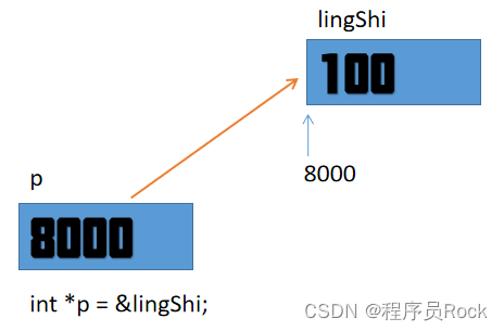
9.指针(上)

Quickly generate illustrations

3. C language uses algebraic cofactor to calculate determinant
Mortal immortal cultivation pointer-1

Service ability of Hongmeng harmonyos learning notes to realize cross end communication
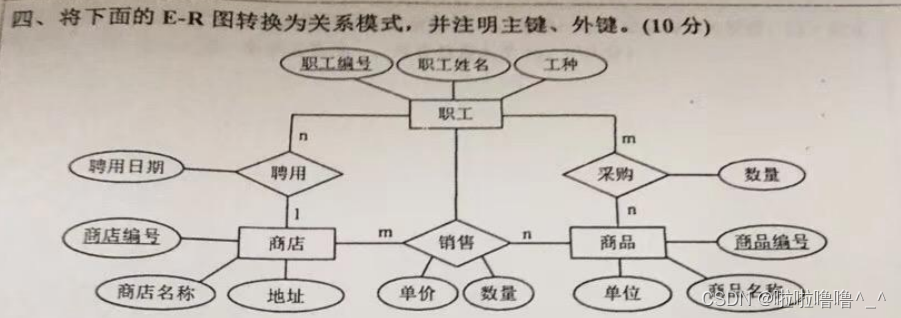
TYUT太原理工大学2022数据库大题之E-R图转关系模式

魏牌:产品叫好声一片,但为何销量还是受挫
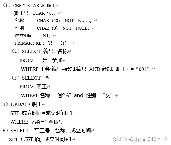
TYUT太原理工大学2022数据库大题之数据库操作

View UI plus released version 1.3.0, adding space and $imagepreview components

2. Preliminary exercises of C language (2)
随机推荐
TYUT太原理工大学往年数据库简述题
最新坦克大战2022-全程开发笔记-3
7. Relationship between array, pointer and array
稻 城 亚 丁
更改VS主题及设置背景图片
学编程的八大电脑操作,总有一款你不会
【九阳神功】2016复旦大学应用统计真题+解析
Tyut Taiyuan University of technology 2022 "Mao Gai" must be recited
IPv6 experiment
用栈实现队列
Share a website to improve your Aesthetics
Wei Pai: the product is applauded, but why is the sales volume still frustrated
3. Number guessing game
MPLS experiment
Common method signatures and meanings of Iterable, collection and list
Change vs theme and set background picture
4.分支语句和循环语句
8.C语言——位操作符与位移操作符
View UI plus released version 1.3.1 to enhance the experience of typescript
View UI plus releases version 1.1.0, supports SSR, supports nuxt, and adds TS declaration files