当前位置:网站首页>Simple query cost estimation
Simple query cost estimation
2022-07-06 06:39:00 【Huawei cloud developer Alliance】
Abstract : The query engine will select the one with the lowest execution cost among all feasible query access paths .
This article is shared from Huawei cloud community 《 Simple query cost estimation 【 Gauss is not a mathematician this time 】》, author : leapdb.
Query cost estimate —— How to choose an optimal execution path
SQL Life cycle : Lexical analysis (Lex) -> Syntax analysis (YACC) -> Analysis rewrite -> Query optimization ( Logical optimization and physical optimization ) -> Query plan generation -> Query execution .
- Lexical analysis : Describe the lexical analyzer *.l Document management Lex Tool build lex.yy.c, Again by C The compiler generates an executable lexical analyzer . The basic function is to set a bunch of strings according to the reserved keywords and non reserved keywords , Convert to the corresponding identifier (Tokens).
- Syntax analysis : Syntax rule description file *.y the YACC Tool build gram.c, Again by C The compiler generates an executable parser . The basic function is to put a bunch of identifiers (Tokens) According to the set grammar rules , Into the original syntax tree .
- Analysis rewrite : Query analysis transforms the original syntax tree into a query syntax tree ( Various transform); Query rewriting is based on pg_rewrite Rules in rewrite tables and views , Finally, we get the query syntax tree .
- Query optimization : After logical optimization and physical optimization ( Generate the optimal path ).
- Query plan generation : Transform the optimal query path into a query plan .
- Query execution : Execute the query plan through the executor to generate the result set of the query .
In the physical optimization stage , The same one SQL Statement can produce many kinds of query paths , for example : Multiple tables JOIN operation , Different JOIN Different execution paths are generated sequentially , It also leads to different sizes of intermediate result tuples . The query engine will select the one with the lowest execution cost among all feasible query access paths .
Usually we rely on COST = COST(CPU) + COST(IO) This formula is used to select the optimal execution plan . here The main problem is how to determine the number of tuples that satisfy a certain condition , The basic method is based on statistical information and certain statistical models . The query cost of a condition = tuple_num * per_tuple_cost.
The main statistical information is pg_class Medium relpages and reltuples, as well as pg_statistics Medium distinct, nullfrac, mcv, histgram etc. .
Why do you need these statistics , Is this enough ?
Statistics are collected from analyze Command to pass random Part of the sample data collected randomly . We turn it into a mathematical problem : Given a constant array, what data characteristics can be analyzed ? Find the rules, huh .
What you can think of with the most simple mathematical knowledge is :
- Is it an empty array
- Is it a constant array
- Is it right? unique No repetition
- Is it orderly
- Is it monotonous , Isochromatic , Equivalency
- What are the most frequent numbers
- Distribution law of data ( The data growth trend is depicted in the dotted way )
anything else ? This is a question worth thinking about .
How to estimate query cost based on statistical information
Statistics are inaccurate , unreliable , Two reasons :
- The statistics are only from part of the sampled data , Can not accurately describe the global characteristics .
- Statistics are historical data , The actual data may change at any time .
How to design a mathematical model , Use unreliable Statistics , Estimate the query cost as accurately as possible , Is a very interesting thing . Next, we will introduce one by one through specific examples .
The main content comes from the following links , We mainly interpret it in detail .
PostgreSQL: Documentation: 14: Chapter 72. How the Planner Uses Statistics
PostgreSQL: Documentation: 14: 14.1. Using EXPLAIN
The simplest table row count estimate ( Use relpages and reltuples)
SELECT relpages, reltuples FROM pg_class WHERE relname = 'tenk1'; --- Sampling estimation has 358 A page ,10000 Bar tuple
 relpages | reltuples
----------+-----------
      358 |     10000

EXPLAIN SELECT * FROM tenk1; --- Query and estimate that the table has 10000 Bar tuple
                         QUERY PLAN
-------------------------------------------------------------
 Seq Scan on tenk1  (cost=0.00..458.00 rows=10000 width=244)
【 reflection 】 Query estimated in the plan rows=10000 Directly pg_class->reltuples Do you ?
Statistics are historical data , The number of tuples in the table changes at any time . for example :analyze There are... During data sampling 10 A page , There is 50 Bar tuple ; The actual implementation includes 20 A page , How many tuples are possible ? Think about it with your most simple emotion , Probably 100 Are the tuples correct ?
The estimation method of table size is in function estimate_rel_size -> table_relation_estimate_size -> heapam_estimate_rel_size in .
- First, calculate the actual number of pages by the size of the physical file of the table actual_pages = file_size / BLOCKSIZE
- Calculate the tuple density of the page
a. If relpages Greater than 0,density = reltuples / (double) relpages
b. If relpages It's empty ,density = (BLCKSZ - SizeOfPageHeaderData) / tuple_width, Page size / Tuple width . - Estimate the number of table tuples = Page tuple density * Actual pages = density * actual_pages
therefore , Estimate rows Of 10000 = (10000 / 358) * 358, Historical page density * Number of new pages , To calculate the current number of tuples .
The simplest range comparison ( Use histogram )
SELECT histogram_bounds FROM pg_stats WHERE tablename='tenk1' AND attname='unique1';
histogram_bounds
------------------------------------------------------
{0,993,1997,3050,4040,5036,5957,7057,8029,9016,9995}
EXPLAIN SELECT * FROM tenk1 WHERE unique1 < 1000; --- Estimate less than 1000 There are 1007 strip
QUERY PLAN
--------------------------------------------------------------------------------
Bitmap Heap Scan on tenk1 (cost=24.06..394.64 rows=1007 width=244)
Recheck Cond: (unique1 < 1000)
-> Bitmap Index Scan on tenk1_unique1 (cost=0.00..23.80 rows=1007 width=0)
Index Cond: (unique1 < 1000)The query engine queries the syntax tree WHERE The comparison condition is identified in the clause , Until then pg_operator Based on the operator and data type oprrest by scalarltsel, This is the cost estimation function of the less than operator of the general scalar data type . In the end scalarineqsel -> ineq_histogram_selectivity Histogram cost estimation in .
stay PG The contour histogram is used in , It's also called equal frequency histogram . Divide the sample range into N Some subintervals of equal parts , Take the boundary values of all subintervals , Form a histogram .
Use : When used, it is considered as subinterval ( Also called bucket ) The values in are linearly monotonically distributed , It is also considered that the coverage of the histogram is the range of the entire data column . therefore , Just calculate the proportion in the histogram , It is the proportion in the total .
【 reflection 】 Are the above two assumptions reliable ? Is there a more reasonable way ?
 Selection rate  = ( Total number of barrels in front  +  The range of the target value in the current bucket  /  The range of the current bucket ) /  Total number of barrels
selectivity = (1 + (1000 - bucket[2].min) / (bucket[2].max - bucket[2].min)) / num_buckets
            = (1 + (1000 - 993) / (1997 - 993)) / 10
            = 0.100697
 Estimate the number of tuples  =  Number of base table tuples  *  Conditional selection rate
rows = rel_cardinality * selectivity
     = 10000 * 0.100697
     = 1007  (rounding off)
The simplest equivalent comparison ( Use MCV)
SELECT null_frac, n_distinct, most_common_vals, most_common_freqs FROM pg_stats WHERE tablename='tenk1' AND attname='stringu1';
null_frac | 0
n_distinct | 676
most_common_vals | {EJAAAA,BBAAAA,CRAAAA,FCAAAA,FEAAAA,GSAAAA,JOAAAA,MCAAAA,NAAAAA,WGAAAA}
most_common_freqs | {0.00333333,0.003,0.003,0.003,0.003,0.003,0.003,0.003,0.003,0.003}
EXPLAIN SELECT * FROM tenk1 WHERE stringu1 = 'CRAAAA'; ---
QUERY PLAN
----------------------------------------------------------
Seq Scan on tenk1 (cost=0.00..483.00 rows=30 width=244)
Filter: (stringu1 = 'CRAAAA'::name)The query engine queries the syntax tree WHERE The comparison condition is identified in the clause , Until then pg_operator Based on the operator and data type oprrest by eqsel, This is the cost estimation function of the general equivalent comparison operator . In the end eqsel_internal -> var_eq_const In the middle of MCV Cost estimation .
MCV It is the highest number of repetitions in the sample 100 Composition , And calculate the proportion of each value in the sample . When using , Simply think that this proportion is the proportion in the overall situation .
【 reflection 】 The proportion in the sample is simply regarded as the proportion in the overall situation , Is that reasonable ? Is there a better way ?
CRAAAA be located MCV No 3 term , The proportion is 0.003
selectivity = mcf[3]
            = 0.003
rows = 10000 * 0.003
     = 30
Next , We are looking at one who is not MCV Equivalence comparison in .
EXPLAIN SELECT * FROM tenk1 WHERE stringu1 = 'xxx'; --- Search does not exist in MCV The value in
                        QUERY PLAN
----------------------------------------------------------
 Seq Scan on tenk1  (cost=0.00..483.00 rows=15 width=244)
   Filter: (stringu1 = 'xxx'::name)
Usually MCV For equivalence comparison , Histograms are used for range comparison .“ There is no in MCV The value in ”, Think of them as share “ There is no in MCV The probability of ”, namely : Selection rate = (1 - MCV Sum of probability ) / ( be not in MCV Of value distinct Number ).
【 reflection 】 This judgment is not MCV Is the method in reasonable ? Is there a better way ?
selectivity = (1 - sum(mvf)) / (num_distinct - num_mcv)
            = (1 - (0.00333333 + 0.003 + 0.003 + 0.003 + 0.003 + 0.003 +
                    0.003 + 0.003 + 0.003 + 0.003)) / (676 - 10)
            = 0.0014559
rows = 10000 * 0.0014559
     = 15  (rounding off)
The more complicated range is ( Use at the same time MCV And histogram )
front unique < 1000 Example , stay scalarineqsel Only the histogram is used in the function , Because unique Column has no duplicate value , There is no such thing as MCV. Now let's use a not unique Let's take a look at the range comparison .
This scope consists of two parts , The value with more repetitions ( stay MCV in ) and A value that repeats less ( Cover in the square diagram ), And because the histogram is calculated without MCV Value , therefore MCV And histogram are independent of each other and can be used in combination .
SELECT null_frac, n_distinct, most_common_vals, most_common_freqs FROM pg_stats WHERE tablename='tenk1' AND attname='stringu1';
null_frac | 0
n_distinct | 676
most_common_vals | {EJAAAA,BBAAAA,CRAAAA,FCAAAA,FEAAAA,GSAAAA,JOAAAA,MCAAAA,NAAAAA,WGAAAA}
most_common_freqs | {0.00333333,0.003,0.003,0.003,0.003,0.003,0.003,0.003,0.003,0.003}
SELECT histogram_bounds FROM pg_stats WHERE tablename='tenk1' AND attname='stringu1';
histogram_bounds
--------------------------------------------------------------------------------
{AAAAAA,CQAAAA,FRAAAA,IBAAAA,KRAAAA,NFAAAA,PSAAAA,SGAAAA,VAAAAA,XLAAAA,ZZAAAA}
EXPLAIN SELECT * FROM tenk1 WHERE stringu1 < 'IAAAAA'; --- Find one that does not exist in MCV The value in
QUERY PLAN
------------------------------------------------------------
Seq Scan on tenk1 (cost=0.00..483.00 rows=3077 width=244)
Filter: (stringu1 < 'IAAAAA'::name)Less than IAAAAA The value of the MCV There are former 6 individual , So put their frac Add up , Is less than IAAAAA And the probability of people who repeat more times
selectivity = sum(relevant mvfs)
            = 0.00333333 + 0.003 + 0.003 + 0.003 + 0.003 + 0.003
            = 0.01833333
Another part is less than IAAAAA But the probability of people who repeat less The range can be calculated by histogram . Use... In the front unique1 Column for equivalence comparison , because unique Constraint column does not exist MCV, Only histograms . therefore , Only calculating the percentage of bucket coverage in the histogram is the selection rate . Here we have to consider falling into The overall percentage of the median in the histogram histogram_fraction = 1 - sum(mcv_frac), Coverage percentage of histogram bucket * The overall proportion of the whole histogram is the selection rate in the histogram .
selectivity = mcv_selectivity + histogram_selectivity * histogram_fraction
            = 0.01833333 + ((2 + ('IAAAAA'-'FRAAAA')/('IBAAAA'-'FRAAAA')) / 10) * (1 - sum(mvfs))
            = 0.01833333 + 0.298387 * 0.96966667
            = 0.307669

rows        = 10000 * 0.307669
            = 3077  (rounding off)
【 reflection 】 In this particular case , from MCV The selection rate calculated in is 0.01833333, Far less than the selection rate calculated from the histogram 0.28933593, Because the distribution of values in this column is slow ( Statistics show MCV These values in appear more frequently than other values , This may be an error caused by sampling ). In most scenarios where there are obviously many duplicate values , from MCV The selection rate calculated in the , Because the occurrence probability of repeated values is relatively accurate .
Example of multi condition joint query
EXPLAIN SELECT * FROM tenk1 WHERE unique1 < 1000 AND stringu1 = 'xxx';
QUERY PLAN
--------------------------------------------------------------------------------
Bitmap Heap Scan on tenk1 (cost=23.80..396.91 rows=1 width=244)
Recheck Cond: (unique1 < 1000)
Filter: (stringu1 = 'xxx'::name)
-> Bitmap Index Scan on tenk1_unique1 (cost=0.00..23.80 rows=1007 width=0)
Index Cond: (unique1 < 1000)The calculation of multi conditional selection rate is also very simple , According to the logical operation of the condition itself .
The two conditions are the relation between and , Are independent events , Just multiply .
selectivity = selectivity(unique1 < 1000) * selectivity(stringu1 = 'xxx')
            = 0.100697 * 0.0014559
            = 0.0001466

rows        = 10000 * 0.0001466
            = 1  (rounding off)
A use JOIN Example
EXPLAIN SELECT * FROM tenk1 t1, tenk2 t2
WHERE t1.unique1 < 50 AND t1.unique2 = t2.unique2;
QUERY PLAN
--------------------------------------------------------------------------------------
Nested Loop (cost=4.64..456.23 rows=50 width=488)
-> Bitmap Heap Scan on tenk1 t1 (cost=4.64..142.17 rows=50 width=244)
Recheck Cond: (unique1 < 50)
-> Bitmap Index Scan on tenk1_unique1 (cost=0.00..4.63 rows=50 width=0)
Index Cond: (unique1 < 50)
-> Index Scan using tenk2_unique2 on tenk2 t2 (cost=0.00..6.27 rows=1 width=244)
Index Cond: (unique2 = t1.unique2)unique1 < 50 The constraint is nested-loop join Was previously executed , Still use histogram calculation , Similar to the previous example of simple range lookup , Only this time 50 Fall in the first bucket .
selectivity = (0 + (50 - bucket[1].min)/(bucket[1].max - bucket[1].min))/num_buckets
            = (0 + (50 - 0)/(993 - 0))/10
            = 0.005035

rows        = 10000 * 0.005035
            = 50  (rounding off)
JOIN constraint t1.unique2 = t2.unique2 Estimation of selection rate , Or first pg_operator Search for “ be equal to ” Operator oprjoin, yes eqjoinsel.JOIN Words , Statistics on both sides should be referred to .
SELECT tablename, null_frac,n_distinct, most_common_vals FROM pg_stats
WHERE tablename IN ('tenk1', 'tenk2') AND attname='unique2';

tablename  | null_frac | n_distinct | most_common_vals
-----------+-----------+------------+------------------
 tenk1     |         0 |         -1 |
 tenk2     |         0 |         -1 |
about unique No column MCV, So here we can only rely on distinct and nullfrac To calculate the selection rate .
【*】 Selection rate  =  Multiply the non empty probabilities on both sides , Divide by the maximum JOIN Number of pieces .
selectivity = (1 - null_frac1) * (1 - null_frac2) * min(1/num_distinct1, 1/num_distinct2)
            = (1 - 0) * (1 - 0) / max(10000, 10000)
            = 0.0001
【*】JOIN The function estimation of is the Cartesian product of the input quantities on both sides , Multiply by the selection rate
rows = (outer_cardinality * inner_cardinality) * selectivity
     = (50 * 10000) * 0.0001
     = 50
If there is MCV, The selection rate is calculated in two parts : stay MCV Part of the sum of is not MCV Part of .
More details
Estimation of table size :src/backend/optimizer/util/plancat.c
Estimation of the selection rate of general logical clauses :src/backend/optimizer/path/clausesel.c
Estimation of selection rate of operator function :src/backend/utils/adt/selfuncs.c.
Click to follow , The first time to learn about Huawei's new cloud technology ~
边栏推荐
- SQL Server Manager studio (SSMS) installation tutorial
- Day 246/300 ssh连接提示“REMOTE HOST IDENTIFICATION HAS CHANGED! ”
- Summary of the post of "Web Test Engineer"
- It is necessary to understand these characteristics in translating subtitles of film and television dramas
- Financial German translation, a professional translation company in Beijing
- Delete external table source data
- MySQL5.72.msi安装失败
- Classification des verbes reconstruits grammaticalement - - English Rabbit Learning notes (2)
- [ 英语 ] 语法重塑 之 英语学习的核心框架 —— 英语兔学习笔记(1)
- 专业论文翻译,英文摘要如何写比较好
猜你喜欢
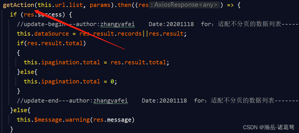
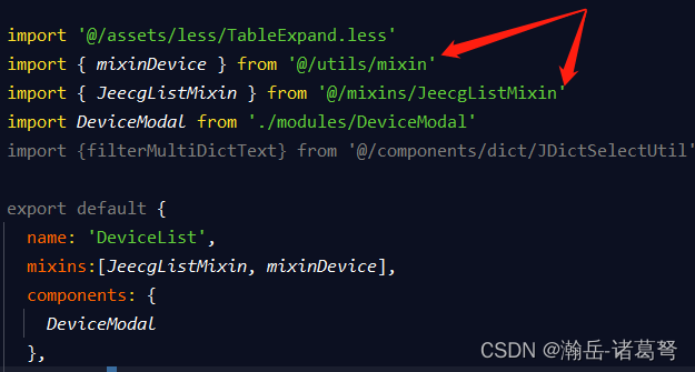
基于JEECG-BOOT的list页面的地址栏参数传递
Transfert des paramètres de la barre d'adresse de la page de liste basée sur jeecg - boot
![[English] Verb Classification of grammatical reconstruction -- English rabbit learning notes (2)](/img/3c/c25e7cbef9be1860842e8981f72352.png)
[English] Verb Classification of grammatical reconstruction -- English rabbit learning notes (2)
Mise en œuvre d’une fonction complexe d’ajout, de suppression et de modification basée sur jeecg - boot
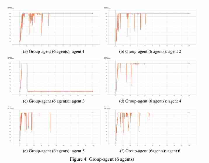
University of Manchester | dda3c: collaborative distributed deep reinforcement learning in swarm agent systems
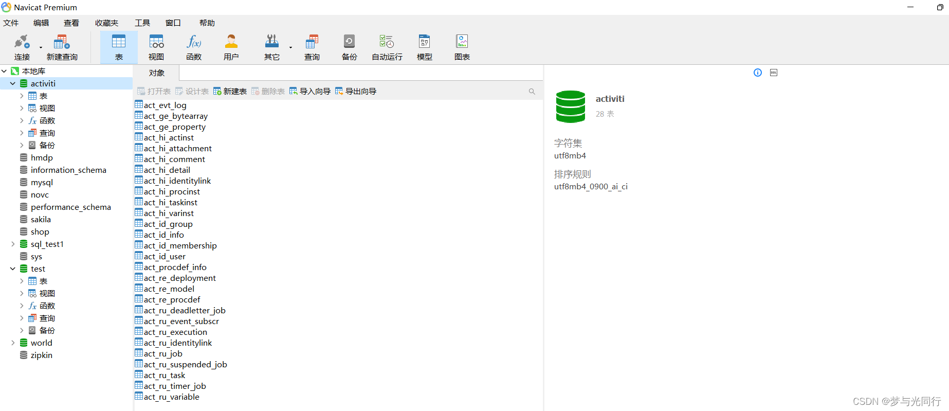
Avtiviti创建表时报错:Error getting a new connection. Cause: org.apache.commons.dbcp.SQLNestedException
Oscp raven2 target penetration process
Suspended else
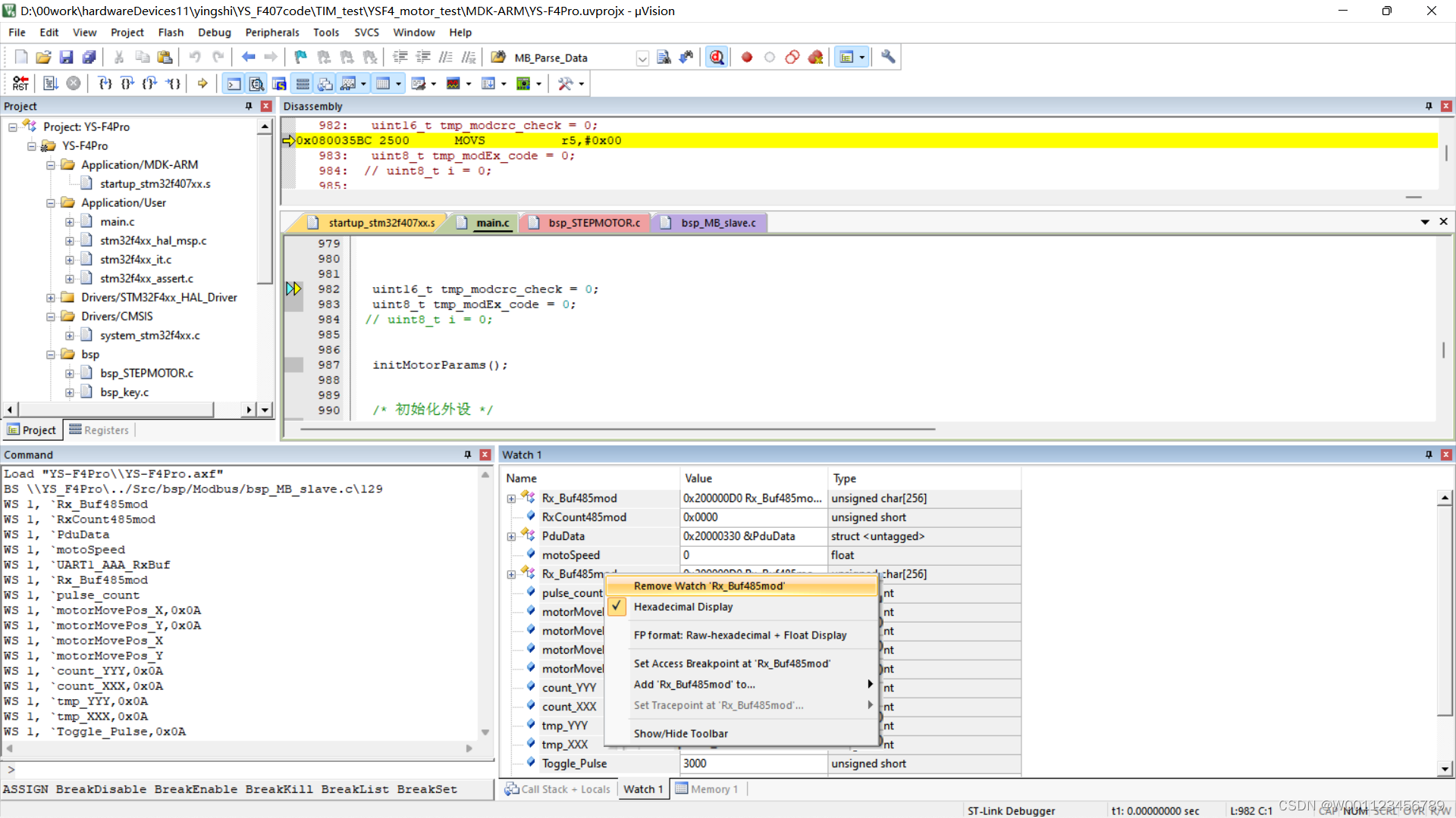
Delete the variables added to watch1 in keil MDK
Biomedical English contract translation, characteristics of Vocabulary Translation
随机推荐
[English] Grammar remodeling: the core framework of English Learning -- English rabbit learning notes (1)
CS certificate fingerprint modification
Summary of the post of "Web Test Engineer"
Simulation volume leetcode [general] 1314 Matrix area and
Phishing & filename inversion & Office remote template
[mqtt from getting started to improving series | 01] quickly build an mqtt test environment from 0 to 1
机器学习植物叶片识别
记一个基于JEECG-BOOT的比较复杂的增删改功能的实现
查询字段个数
Traffic encryption of red blue confrontation (OpenSSL encrypted transmission, MSF traffic encryption, CS modifying profile for traffic encryption)
Black cat takes you to learn UFS protocol Chapter 4: detailed explanation of UFS protocol stack
Day 245/300 JS forEach 多层嵌套后数据无法更新到对象中
SQL Server manager studio(SSMS)安装教程
Avtiviti创建表时报错:Error getting a new connection. Cause: org.apache.commons.dbcp.SQLNestedException
Day 239/300 注册密码长度为8~14个字母数字以及标点符号至少包含2种校验
JDBC requset corresponding content and function introduction
Simulation volume leetcode [general] 1447 Simplest fraction
MySQL5.72. MSI installation failed
自动化测试环境配置
基于JEECG-BOOT制作“左树右表”交互页面