当前位置:网站首页>Advanced opencv:bgr pixel intensity map
Advanced opencv:bgr pixel intensity map
2022-07-05 10:09:00 【woshicver】
Introduce
up to now , In our advanced OpenCV tutorial , We have :
Understand the concept of contrast .
Understand the concept of histogram equalization .
Implement contrast enhancement on grayscale images .
Draw the pixel histogram of gray-scale image .
However , as everyone knows , Our world is made up of many, many colors . Now we will try to analyze the contrast and pixel intensity of color images , That is, the image with color channel .
In order to promote this special advanced OpenCV Learning experience , We will use this link (https://wallpaperaccess.com/cool-outer-space) Downloaded images . perhaps , You can save the image found below .

Learn about color images
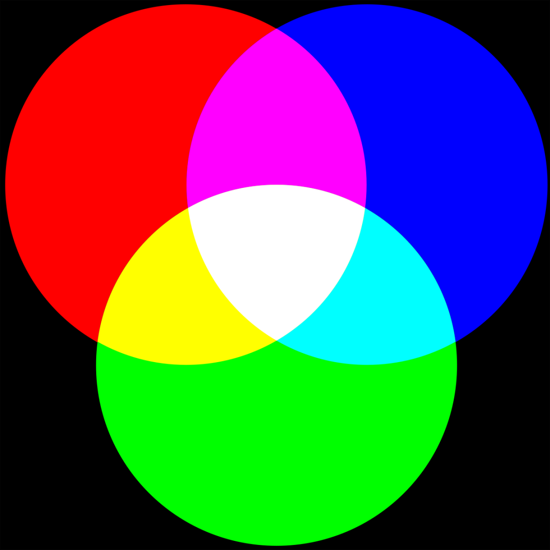
If you have read our previous articles , If I remember correctly , We learned about advanced OpenCV Use BGR Color channel , instead of RGB. You will find that the red and blue channels have been exchanged .
As shown in the figure above , There are many colors that are eye-catching and eye-catching . These colors with different hues are the result of mixing color channels .
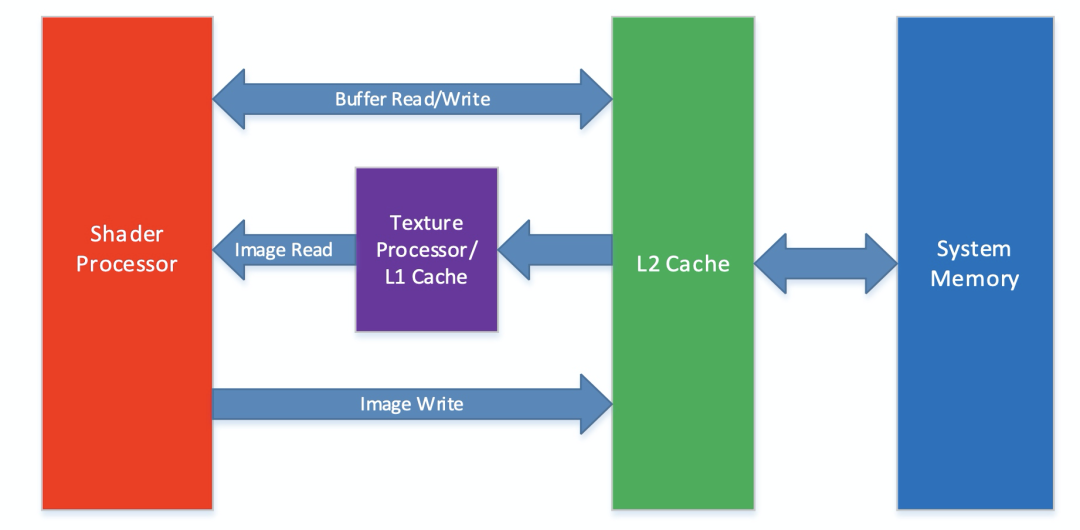
There are three color channels in this image :
Blue
green
Red
It is through the mixing of these colors , Can appear belong to the secondary color of chromatography and many other colors .
Gain image insight
The first and most important step is to import the necessary packages into our python Script , Then we load the image into our system RAM in . This will be done by OpenCV Provided by the package imread() Method to accomplish :
import cv2
import numpy as np
from matplotlib import pyplot as plt
img = cv2.imread('C:/Users/Shivek/Pictures/Picture1.jpg')
The output of the above code block will be shown below :
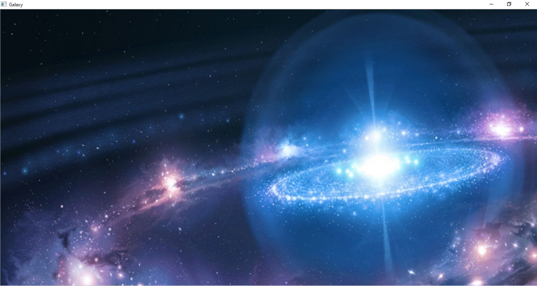
As one may observe , The image is too big to be displayed in full size on my screen . however , We will not reduce the size of the image . This is because we want to know more about the properties and related information of pixels .
First , Let's see Image The shape of the (NumPy Array ):
print(image.shape)The output of the above code line will be shown below :
After carefully checking this information tuple , It will be decrypted as follows :
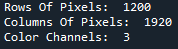
The color channel is BGR-NOT RGB. Next , Let's see The size of the image —— Size tells us the total number of pixels that make up the entire image .
print(image.size)Output :
6912000There are more than 600 Mega pixels .
Let's look at the first pixel in the image . This is the pixel in the first row and the first column .
print(image[0][0])
its BGR Values, respectively 22、15 and 6.
Now let's move on :BGR Pixel count diagram .
BGR Pixel intensity line graph
Because every pixel in our image contains 3 A color channel , So we will need to traverse all pixels 3 Time , Each time from B、G and R Select the value in the channel . To do this , Can be for Circulation and enumerate() Function in combination with .
We may already know , enumerate() Function will allow us to traverse a fixed number of elements , And automatically record the number of each element .
We will use MatPlotLib The package obtains the visual effect of pixel intensity and count in the form of line graph .
colors = ('blue','green','red')
label = ("Blue", "Green", "Red")
for count,color in enumerate(colors):
    histogram = cv2.calcHist([image],[count],None,[256],[0,256])
    plt.plot(histogram,color = color, label=label[count]+str(" Pixels"))
The line by line explanation of the above code block is as follows :
In the following code line , We created a tuple , It contains the colors of three different lines of the figure . Because of 3 Sub iteration , Each iteration will choose a different color , So we can see on the chart BGR Pattern .
Color =(' Blue ',' green ',' Red ')
thereafter , Let's continue to create a tuple , It contains the corresponding labels of the chart legend . Again , At each iteration , A label will be selected to mark the corresponding color of the graphic . These labels will be included in the legend of the chart , We will see in the following lines .
label = ("Blue", "Green", "Red")In order to facilitate graphic generation , We have a for-enumerate loop , This loop will be executed to select each required item from the pixel array and tuple , On these projects , They will be drawn as a line chart on the same canvas .
for count,color in enumerate(colors):
    histogram = cv2.calcHist([image],[count],None,[256],[0,256])
    plt.plot(histogram,color = color, label=label[count]+str(" Pixels"))
for The lines of code in the loop are as follows :
histogram = cv2.calcHist([image],[count],None,[256],[0,256])We will use OpenCV In bag calcHist() Method , This method will obtain the histogram of pixel intensity , As we know in the previous article . We pass in the following parameters :
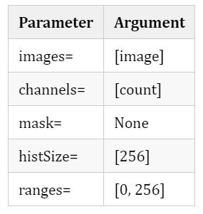
In order to draw graphics , We use MatPlotLib Provided by the package plot() Method , As shown below :
plt.plot(histogram, color=color, label=label[count]+str(" Pixels"))We pass in the data to be plotted , Then the appropriate color . Assign a label to the graph , And according to for Iterate over the corresponding label in the index tuple . We will “ Pixels ” Append to tag name , So that the viewer can clearly see the completed graphics .
Before displaying the chart to the end user , We added some elements to the diagram , for example :
title .
Y The label of the shaft .
X The label of the shaft .
A legend .
To end processing , We use MatPlotLib Provided by the package show() Method to display the visual effect on the screen .
plt.title("Histogram Showing Number Of Pixels Belonging To Respective Pixel Intensity", color="crimson")
plt.ylabel("Number Of Pixels", color="crimson")
plt.xlabel("Pixel Intensity", color="crimson")
plt.legend(numpoints=1, loc="best")
plt.show()
The final BGR The pixel intensity line graph will be as follows :
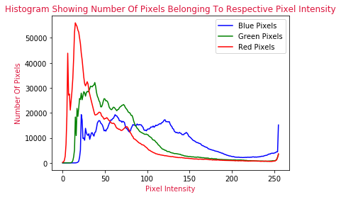
The above visual display tells us exactly how the pixels are distributed in the original color image . What makes up our image 600 ten thousand + The position of pixels can be summarized in the above line graph .
Most of our pixels are on the left side of the image , As you can see from the diagram , The image is blue from the middle to the right , As shown by the blue pixel intensity line . Blue pixel intensity lines dominate these areas - If people look at images , That's true :
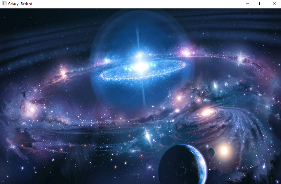
Please note how the full image fits my computer screen - This is because I adjusted its size .
A very interesting fact is , Although I have adjusted the size of the image , But if I want to create a pixel intensity map on the resized image , Then compared with the original image ,BGR The gradient of the graph is no different —— It just shrinks in size or “ scale ”.
Conclusion
In this paper , We studied :
stay Python Used in programming languages OpenCV Understand color images
BGR Color channel
Use Python Medium MatPlotLib Bao Jiang BGR Pixels are mapped to BGR Pixel intensity line graph
* END *
If you see this , Show that you like this article , Please forward 、 give the thumbs-up . WeChat search 「uncle_pn」, Welcome to add Xiaobian wechat 「 woshicver」, Update a high-quality blog post in your circle of friends every day .
↓ Scan QR code and add small code ↓

边栏推荐
- Windows uses commands to run kotlin
- Charm of code language
- QT timer realizes dynamic display of pictures
- How to correctly evaluate video image quality
- 90%的人都不懂的泛型,泛型的缺陷和应用场景
- [NTIRE 2022]Residual Local Feature Network for Efficient Super-Resolution
- idea用debug调试出现com.intellij.rt.debugger.agent.CaptureAgent,导致无法进行调试
- How do enterprises choose the appropriate three-level distribution system?
- Kotlin compose and native nesting
- Tianlong Babu TLBB series - about items dropped from packages
猜你喜欢
The writing speed is increased by dozens of times, and the application of tdengine in tostar intelligent factory solution
mysql80服务不启动
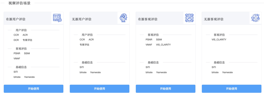
How to correctly evaluate video image quality
双容水箱液位模糊PID控制系统设计与仿真(Matlab/Simulink)
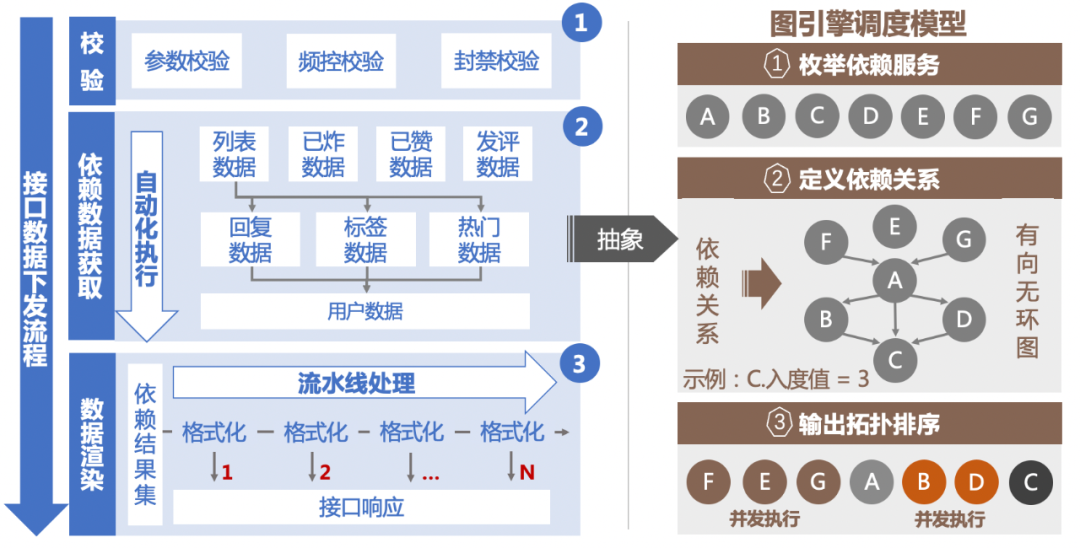
Design and exploration of Baidu comment Center
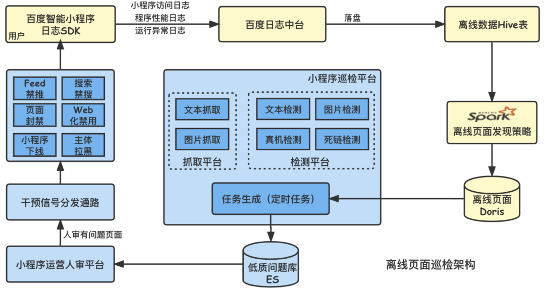
百度智能小程序巡檢調度方案演進之路

盗版DALL·E成梗图之王?日产5万张图像,挤爆抱抱脸服务器,OpenAI勒令改名
Mobile heterogeneous computing technology GPU OpenCL programming (Advanced)
. Net delay queue
【小技巧】获取matlab中cdfplot函数的x轴,y轴的数值
随机推荐
Node red series (29): use slider and chart nodes to realize double broken line time series diagram
H. 265 introduction to coding principles
如何获取GC(垃圾回收器)的STW(暂停)时间?
Online chain offline integrated chain store e-commerce solution
Android SQLite database encryption
解决idea调试过程中liquibase – Waiting for changelog lock….导致数据库死锁问题
QT event filter simple case
Is it really reliable for AI to make complex decisions for enterprises? Participate in the live broadcast, Dr. Stanford to share his choice | qubit · viewpoint
硬核,你见过机器人玩“密室逃脱”吗?(附代码)
【 conseils 】 obtenir les valeurs des axes X et y de la fonction cdfplot dans MATLAB
How to get the STW (pause) time of GC (garbage collector)?
盗版DALL·E成梗图之王?日产5万张图像,挤爆抱抱脸服务器,OpenAI勒令改名
ArcGIS Pro creating features
Coordinate system of view
小程序启动性能优化实践
Design and exploration of Baidu comment Center
天龙八部TLBB系列 - 关于技能冷却和攻击范围数量的问题
RMS TO EAP通过MQTT简单实现
Generics, generic defects and application scenarios that 90% of people don't understand
让AI替企业做复杂决策真的靠谱吗?参与直播,斯坦福博士来分享他的选择|量子位·视点...