当前位置:网站首页>ML之shap:基于adult人口普查收入二分类预测数据集(预测年收入是否超过50k)利用Shap值对XGBoost模型实现可解释性案例之详细攻略
ML之shap:基于adult人口普查收入二分类预测数据集(预测年收入是否超过50k)利用Shap值对XGBoost模型实现可解释性案例之详细攻略
2022-07-06 06:33:00 【一个处女座的程序猿】
ML之shap:基于adult人口普查收入二分类预测数据集(预测年收入是否超过50k)利用Shap值对XGBoost模型实现可解释性案例之详细攻略
目录
基于adult人口普查收入二分类预测数据集(预测年收入是否超过50k)利用Shap值对XGBoost模型实现可解释性案例
# 5.1、力图可视化分析:可视化单个或多个样本内各个特征贡献度并对比模型预测值——探究误分类样本
基于adult人口普查收入二分类预测数据集(预测年收入是否超过50k)利用Shap值对XGBoost模型实现可解释性案例
1、定义数据集
dtypes_len: 15
| age | workclass | fnlwgt | education | education_num | marital_status | occupation | relationship | race | sex | capital_gain | capital_loss | hours_per_week | native_country | salary |
| 39 | State-gov | 77516 | Bachelors | 13 | Never-married | Adm-clerical | Not-in-family | White | Male | 2174 | 0 | 40 | United-States | <=50K |
| 50 | Self-emp-not-inc | 83311 | Bachelors | 13 | Married-civ-spouse | Exec-managerial | Husband | White | Male | 0 | 0 | 13 | United-States | <=50K |
| 38 | Private | 215646 | HS-grad | 9 | Divorced | Handlers-cleaners | Not-in-family | White | Male | 0 | 0 | 40 | United-States | <=50K |
| 53 | Private | 234721 | 11th | 7 | Married-civ-spouse | Handlers-cleaners | Husband | Black | Male | 0 | 0 | 40 | United-States | <=50K |
| 28 | Private | 338409 | Bachelors | 13 | Married-civ-spouse | Prof-specialty | Wife | Black | Female | 0 | 0 | 40 | Cuba | <=50K |
| 37 | Private | 284582 | Masters | 14 | Married-civ-spouse | Exec-managerial | Wife | White | Female | 0 | 0 | 40 | United-States | <=50K |
| 49 | Private | 160187 | 9th | 5 | Married-spouse-absent | Other-service | Not-in-family | Black | Female | 0 | 0 | 16 | Jamaica | <=50K |
| 52 | Self-emp-not-inc | 209642 | HS-grad | 9 | Married-civ-spouse | Exec-managerial | Husband | White | Male | 0 | 0 | 45 | United-States | >50K |
| 31 | Private | 45781 | Masters | 14 | Never-married | Prof-specialty | Not-in-family | White | Female | 14084 | 0 | 50 | United-States | >50K |
| 42 | Private | 159449 | Bachelors | 13 | Married-civ-spouse | Exec-managerial | Husband | White | Male | 5178 | 0 | 40 | United-States | >50K |
2、数据集预处理
# 2.1、入模特征初步筛选
df.columns
14
# 2.2、目标特征二值化
# 2.3、类别型特征编码数字化
filt_dtypes_len: 13 [('age', 'float32'), ('workclass', 'category'), ('fnlwgt', 'float32'), ('education_Num', 'float32'), ('marital_status', 'category'), ('occupation', 'category'), ('relationship', 'category'), ('race', 'category'), ('sex', 'category'), ('capital_gain', 'float32'), ('capital_loss', 'float32'), ('hours_per_week', 'float32'), ('native_country', 'category')]
# 2.4、分离特征与标签
df_adult_display
| age | workclass | education_num | marital_status | occupation | relationship | race | sex | capital_gain | capital_loss | hours_per_week | native_country | salary | |
| 0 | 39 | State-gov | 13 | Never-married | Adm-clerical | Not-in-family | White | Male | 2174 | 0 | 40 | United-States | 0 |
| 1 | 50 | Self-emp-not-inc | 13 | Married-civ-spouse | Exec-managerial | Husband | White | Male | 0 | 0 | 13 | United-States | 0 |
| 2 | 38 | Private | 9 | Divorced | Handlers-cleaners | Not-in-family | White | Male | 0 | 0 | 40 | United-States | 0 |
| 3 | 53 | Private | 7 | Married-civ-spouse | Handlers-cleaners | Husband | Black | Male | 0 | 0 | 40 | United-States | 0 |
| 4 | 28 | Private | 13 | Married-civ-spouse | Prof-specialty | Wife | Black | Female | 0 | 0 | 40 | Cuba | 0 |
| 5 | 37 | Private | 14 | Married-civ-spouse | Exec-managerial | Wife | White | Female | 0 | 0 | 40 | United-States | 0 |
| 6 | 49 | Private | 5 | Married-spouse-absent | Other-service | Not-in-family | Black | Female | 0 | 0 | 16 | Jamaica | 0 |
| 7 | 52 | Self-emp-not-inc | 9 | Married-civ-spouse | Exec-managerial | Husband | White | Male | 0 | 0 | 45 | United-States | 1 |
| 8 | 31 | Private | 14 | Never-married | Prof-specialty | Not-in-family | White | Female | 14084 | 0 | 50 | United-States | 1 |
| 9 | 42 | Private | 13 | Married-civ-spouse | Exec-managerial | Husband | White | Male | 5178 | 0 | 40 | United-States | 1 |
df_adult
| age | workclass | education_num | marital_status | occupation | relationship | race | sex | capital_gain | capital_loss | hours_per_week | native_country | salary | |
| 0 | 39 | 7 | 13 | 4 | 1 | 1 | 4 | 1 | 2174 | 0 | 40 | 39 | 0 |
| 1 | 50 | 6 | 13 | 2 | 4 | 0 | 4 | 1 | 0 | 0 | 13 | 39 | 0 |
| 2 | 38 | 4 | 9 | 0 | 6 | 1 | 4 | 1 | 0 | 0 | 40 | 39 | 0 |
| 3 | 53 | 4 | 7 | 2 | 6 | 0 | 2 | 1 | 0 | 0 | 40 | 39 | 0 |
| 4 | 28 | 4 | 13 | 2 | 10 | 5 | 2 | 0 | 0 | 0 | 40 | 5 | 0 |
| 5 | 37 | 4 | 14 | 2 | 4 | 5 | 4 | 0 | 0 | 0 | 40 | 39 | 0 |
| 6 | 49 | 4 | 5 | 3 | 8 | 1 | 2 | 0 | 0 | 0 | 16 | 23 | 0 |
| 7 | 52 | 6 | 9 | 2 | 4 | 0 | 4 | 1 | 0 | 0 | 45 | 39 | 1 |
| 8 | 31 | 4 | 14 | 4 | 10 | 1 | 4 | 0 | 14084 | 0 | 50 | 39 | 1 |
| 9 | 42 | 4 | 13 | 2 | 4 | 0 | 4 | 1 | 5178 | 0 | 40 | 39 | 1 |
# 2.5、数据集整体切分
df_len: 32561 ,train_test_index: 30933
X.shape,y.shape: (30933, 12) (30933,)
X_test.shape,y_test.shape: (1628, 12) (1628,)
#3、模型训练与推理
# 3.1、数据集切分
# 3.2、模型建立并训练
# 3.3、模型预测
| age | workclass | education_num | marital_status | occupation | relationship | race | sex | capital_gain | capital_loss | hours_per_week | native_country | y_val_predi | y_val | |
| 11311 | 29 | 4 | 9 | 4 | 1 | 3 | 2 | 0 | 0 | 0 | 60 | 39 | 0 | 0 |
| 12519 | 33 | 4 | 10 | 4 | 3 | 1 | 2 | 1 | 8614 | 0 | 40 | 39 | 1 | 1 |
| 29225 | 27 | 4 | 13 | 4 | 10 | 1 | 4 | 1 | 0 | 0 | 45 | 39 | 0 | 0 |
| 5428 | 22 | 4 | 9 | 2 | 7 | 0 | 4 | 1 | 0 | 0 | 40 | 39 | 0 | 0 |
| 2400 | 32 | 7 | 10 | 4 | 1 | 1 | 2 | 0 | 0 | 0 | 40 | 39 | 0 | 0 |
| 4319 | 45 | 4 | 10 | 2 | 4 | 0 | 4 | 1 | 0 | 0 | 40 | 39 | 1 | 0 |
| 26564 | 43 | 4 | 9 | 2 | 6 | 0 | 4 | 1 | 0 | 0 | 40 | 39 | 0 | 0 |
| 4721 | 60 | 0 | 13 | 2 | 0 | 0 | 4 | 1 | 0 | 0 | 8 | 39 | 0 | 1 |
| 19518 | 29 | 6 | 9 | 2 | 12 | 0 | 4 | 1 | 0 | 0 | 35 | 39 | 0 | 0 |
| 25013 | 33 | 4 | 5 | 2 | 6 | 0 | 4 | 1 | 0 | 0 | 40 | 39 | 0 | 0 |
#4、模型特征重要性解释可视化
#4.1、全局特征重要性可视化
# T1、基于模型本身输出特征重要性
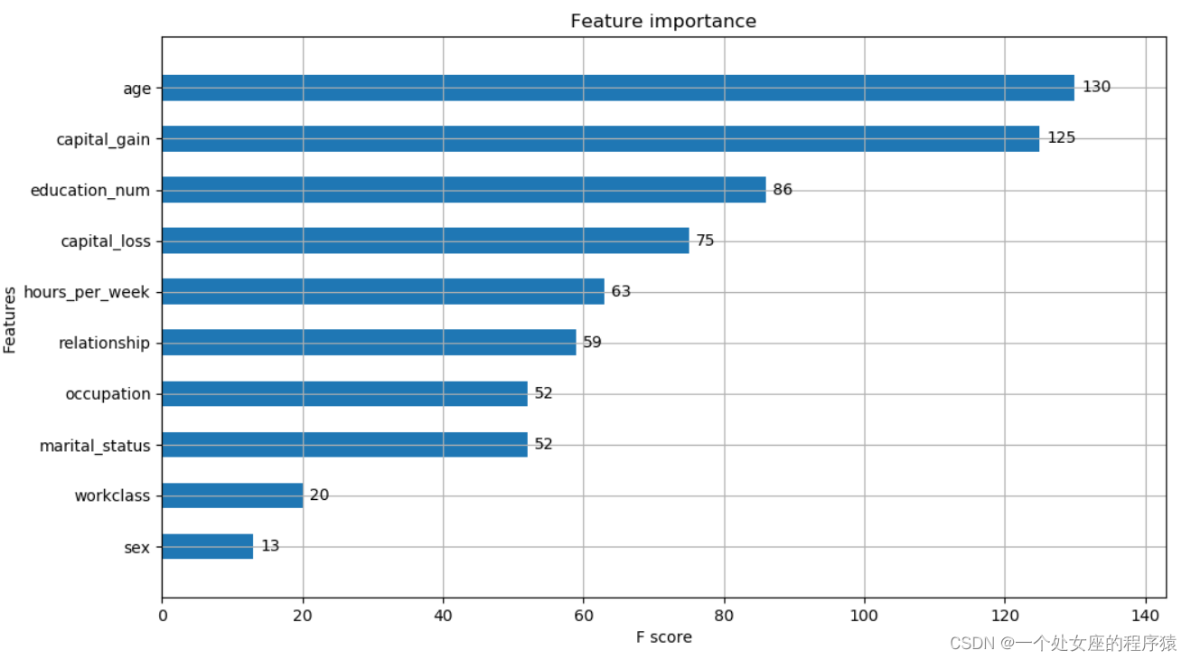
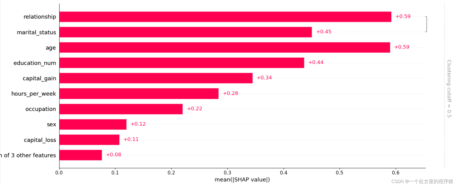
XGBR_importance_dict: [('age', 130), ('capital_gain', 125), ('education_num', 86), ('capital_loss', 75), ('hours_per_week', 63), ('relationship', 59), ('marital_status', 52), ('occupation', 52), ('workclass', 20), ('sex', 13), ('native_country', 10), ('race', 6)]
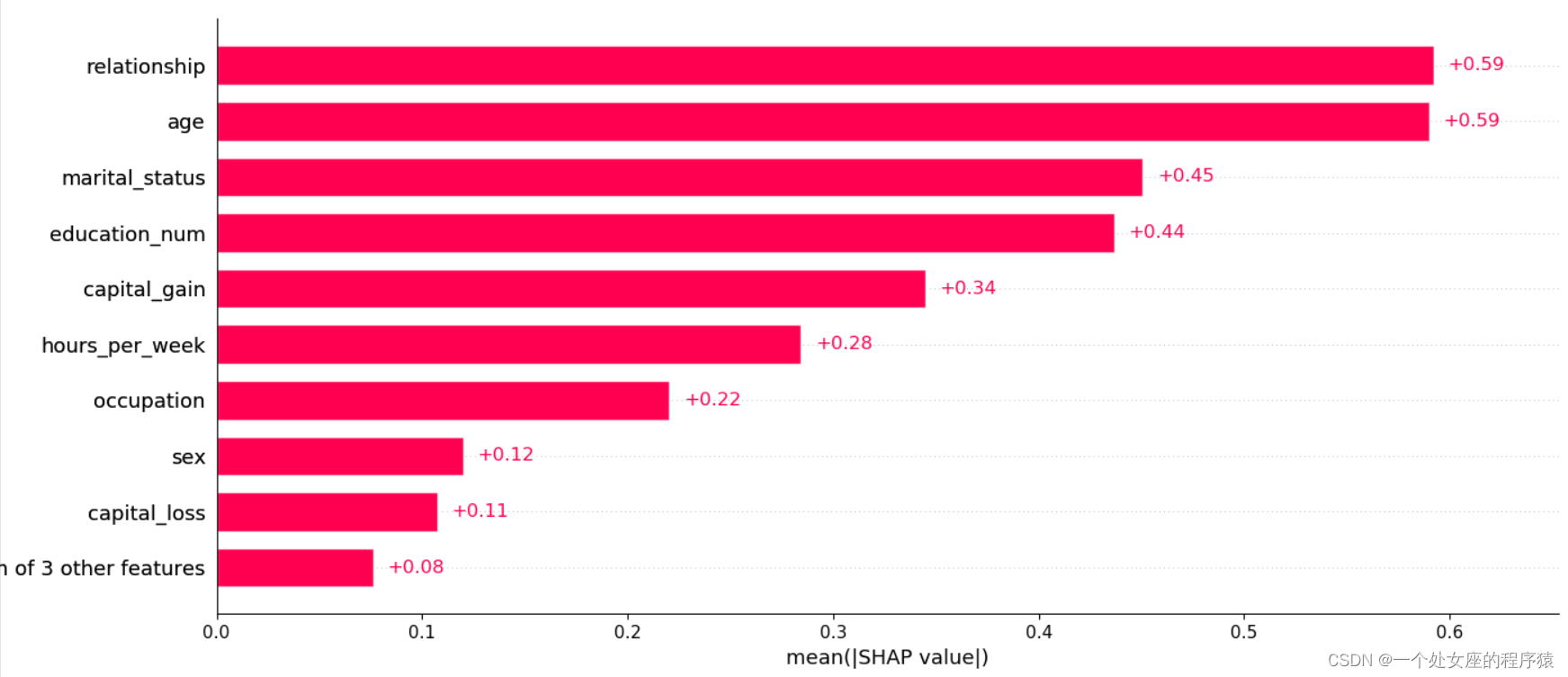
# T2、利用Shap值解释XGBR模型
利用shap自带的函数实现特征贡献性可视化——特征重要性排序与上边类似,但并不相同
# (1)、创建Explainer并计算SHAP值

# T2.1、输出shap.Explanation对象
# T2,2、输出numpy.array数组
shap2exp.values.shape (30933, 12)
 [[ 0.31074238 -0.16607898  0.5617416  ... -0.04660619 -0.09465054
   0.00530914]
 [ 0.34912622 -0.16633348  0.65308005 ... -0.06718991 -0.9804511
   0.00515459]
 [ 0.21971266  0.02263742 -0.299867   ... -0.0583196  -0.09738331
   0.00415599]
 ...
 [-0.48140627  0.07019287 -0.30844492 ... -0.04253047 -0.10924102
   0.00649792]
 [ 0.39729887 -0.2313431  -0.45257783 ... -0.06502013  0.27416423
   0.00587647]
 [ 0.27594262  0.03170239  0.78293955 ... -0.06743324  0.31613
   0.00530914]]
shap2array.shape (30933, 12)
 [[ 0.31074238 -0.16607898  0.5617416  ... -0.04660619 -0.09465054
   0.00530914]
 [ 0.34912622 -0.16633348  0.65308005 ... -0.06718991 -0.9804511
   0.00515459]
 [ 0.21971266  0.02263742 -0.299867   ... -0.0583196  -0.09738331
   0.00415599]
 ...
 [-0.48140627  0.07019287 -0.30844492 ... -0.04253047 -0.10924102
   0.00649792]
 [ 0.39729887 -0.2313431  -0.45257783 ... -0.06502013  0.27416423
   0.00587647]
 [ 0.27594262  0.03170239  0.78293955 ... -0.06743324  0.31613
   0.00530914]]
shap2exp.values与shap2array,两个矩阵否相等: True
# (2)、全样本各特征shap值条形图可视化
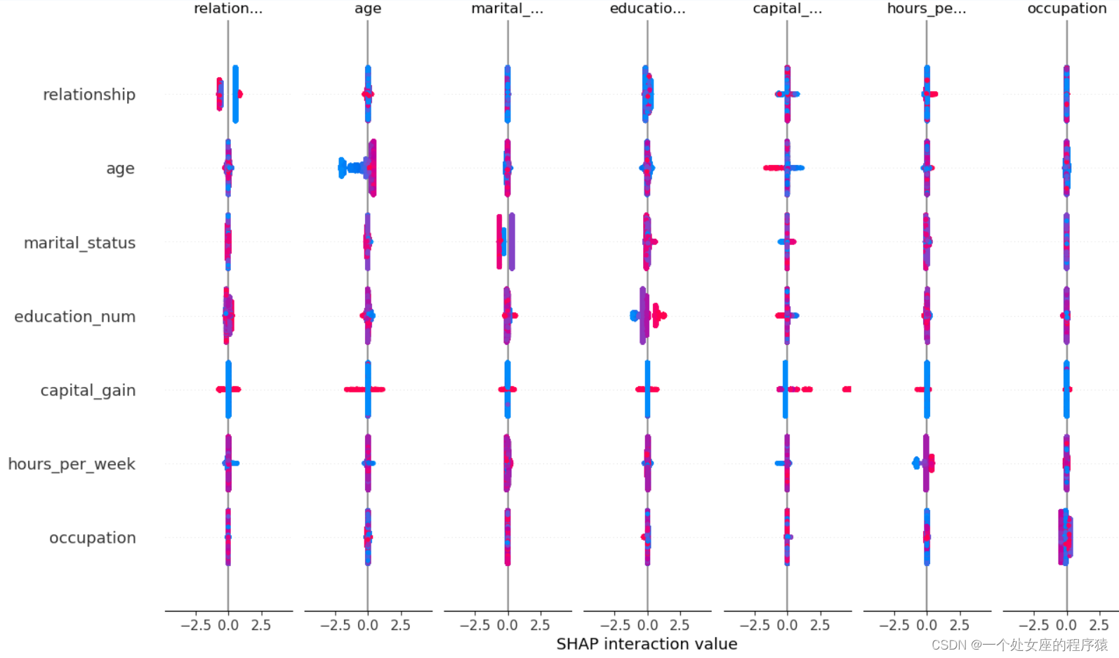
# shap值高阶交互可视化
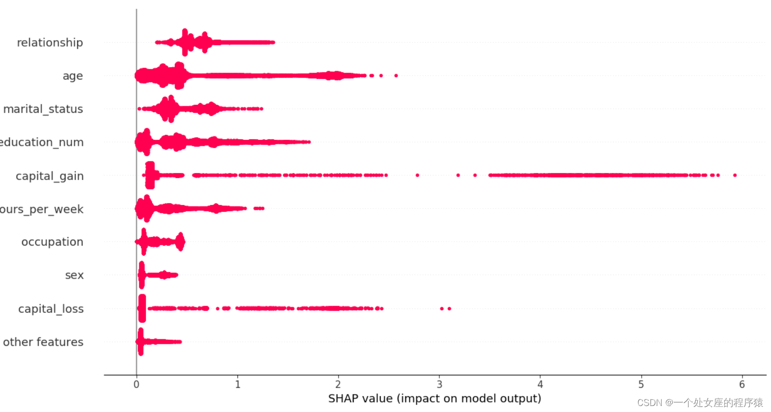
# (3)、全样本各特征shap值蜂群图可视化
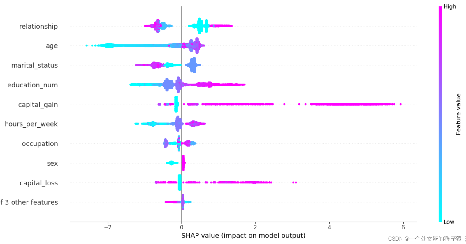
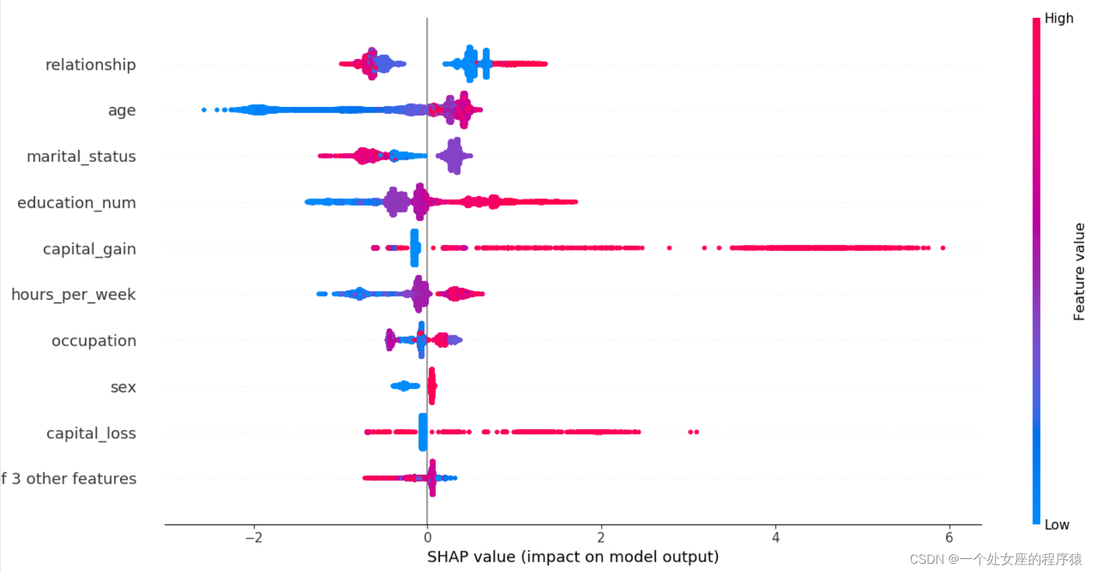
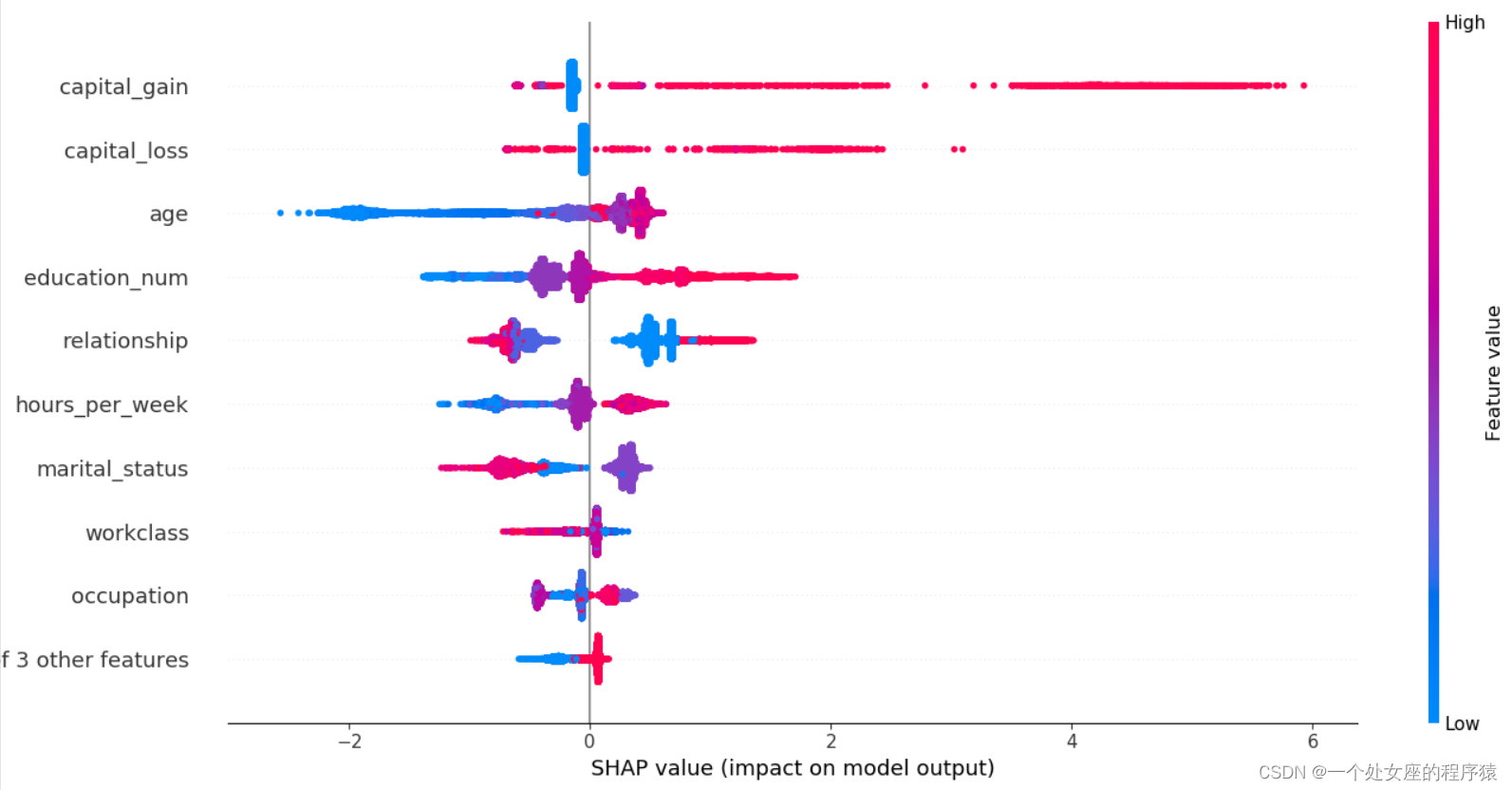
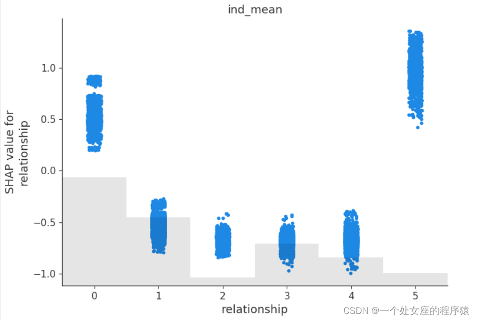
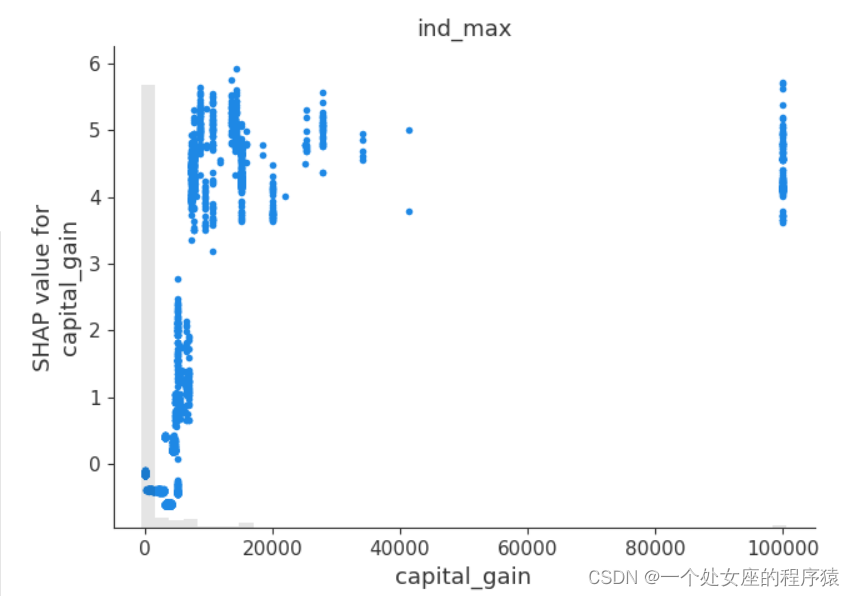
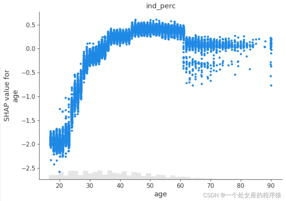
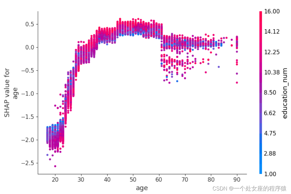
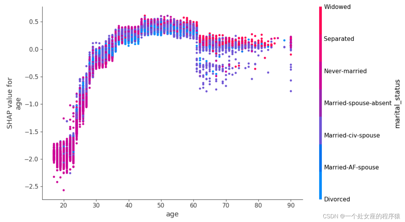
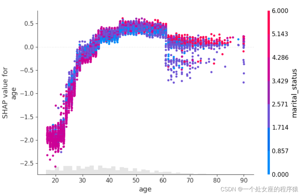
# (4)、全局特征重要性排序散点图可视化
#4.2、局部特征重要性可视化
# (1)、单样本全特征条形图可视化
前测试样本:0
.values =
array([ 0.31074238, -0.16607898,  0.5617416 , -0.58709425, -0.08897061,
       -0.6133537 ,  0.01539118,  0.04758333, -0.3988452 , -0.04660619,
       -0.09465054,  0.00530914], dtype=float32)
.base_values =
-1.3270257
.data =
array([3.900e+01, 7.000e+00, 1.300e+01, 4.000e+00, 1.000e+00, 1.000e+00,
       4.000e+00, 1.000e+00, 2.174e+03, 0.000e+00, 4.000e+01, 3.900e+01])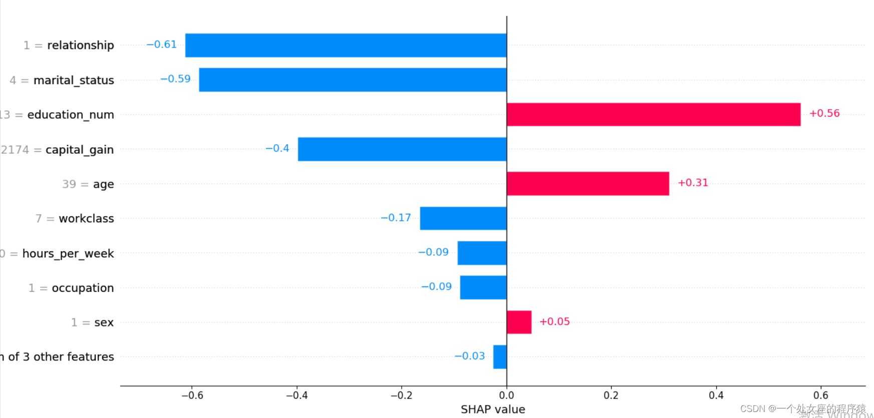
前测试样本:1
.values =
array([ 0.34912622, -0.16633348,  0.65308005,  0.3069151 ,  0.26878497,
        0.5229906 ,  0.01030679,  0.04531586, -0.15429462, -0.06718991,
       -0.9804511 ,  0.00515459], dtype=float32)
.base_values =
-1.3270257
.data =
array([50.,  6., 13.,  2.,  4.,  0.,  4.,  1.,  0.,  0., 13., 39.])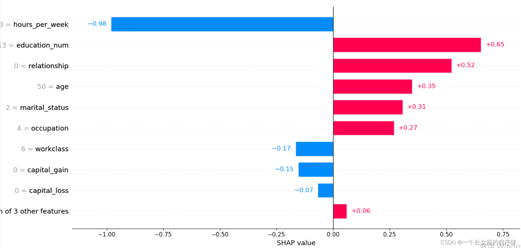
前测试样本:10
.values =
array([ 0.27578622,  0.02686635, -0.0699547 ,  0.2820353 ,  0.3097189 ,
        0.55229187, -0.03686382,  0.05135565, -0.1607191 , -0.06321771,
        0.38190693,  0.02023092], dtype=float32)
.base_values =
-1.3270257
.data =
array([37.,  4., 10.,  2.,  4.,  0.,  2.,  1.,  0.,  0., 80., 39.])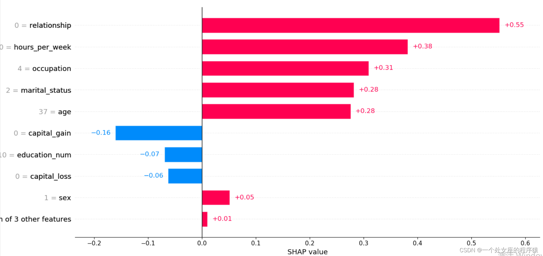
前测试样本:20
.values =
array([ 0.31008577,  0.00316932,  1.3133987 ,  0.16768128,  0.18239255,
        0.6863757 ,  0.00508371,  0.05159741, -0.15813455, -0.06736177,
        0.31327826,  0.01936885], dtype=float32)
.base_values =
-1.3270257
.data =
array([40.,  4., 16.,  2., 10.,  0.,  4.,  1.,  0.,  0., 60., 39.])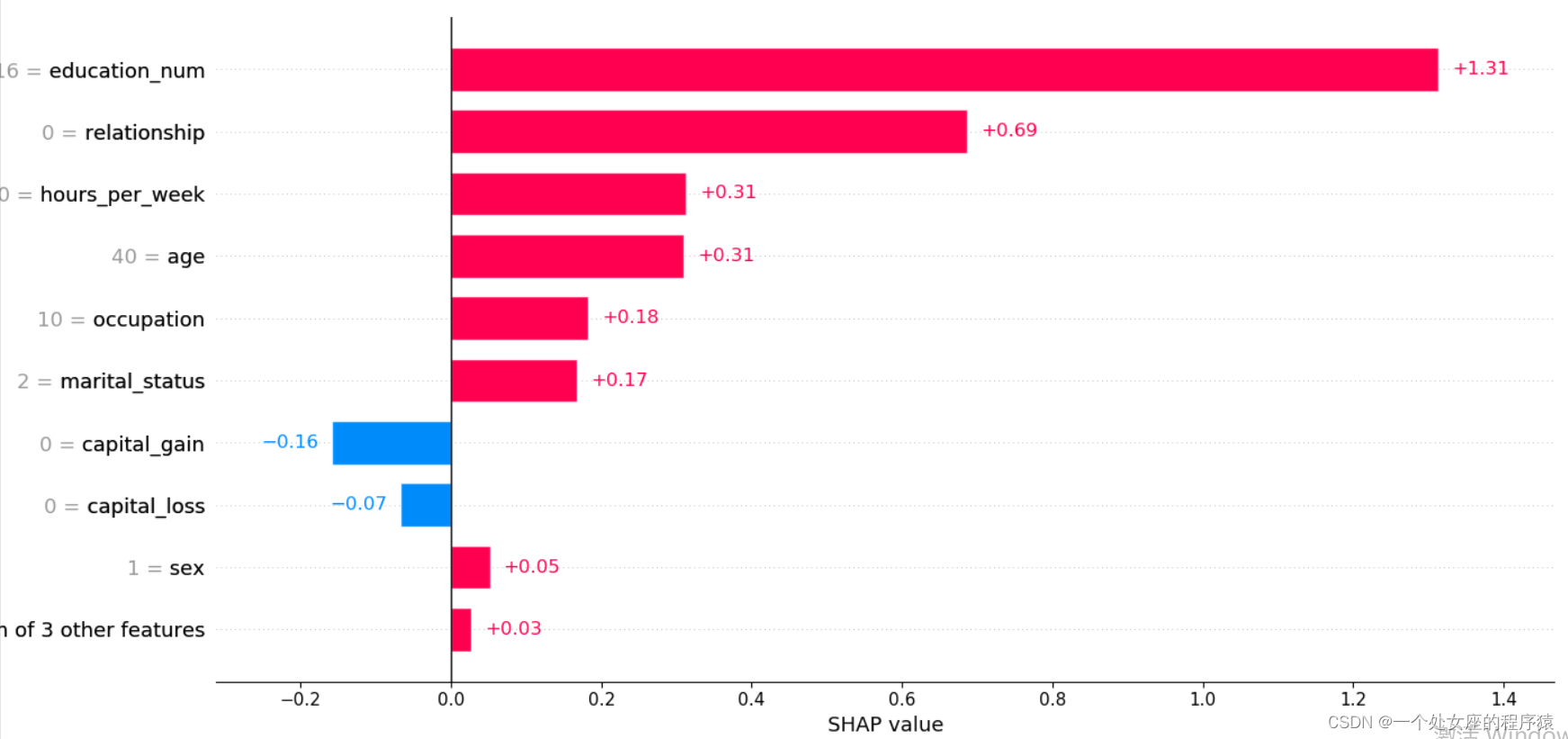
# (2)、单转双特征全样本局部独立图散点图可视化
# (3)、双特征全样本散点图可视化
# 4.3、模型特征筛选
# (1)、基于聚类的shap特征筛选可视化
5、模型预测的可解释性(可主要分析误分类的样本)
提供了预测的细节,侧重于解释单个预测是如何生成的。它可以帮助决策者信任模型,并且解释各个特征是如何影响模型单次的决策。
# 5.1、力图可视化分析:可视化单个或多个样本内各个特征贡献度并对比模型预测值——探究误分类样本
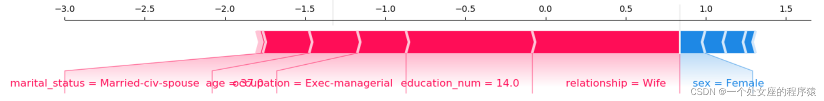
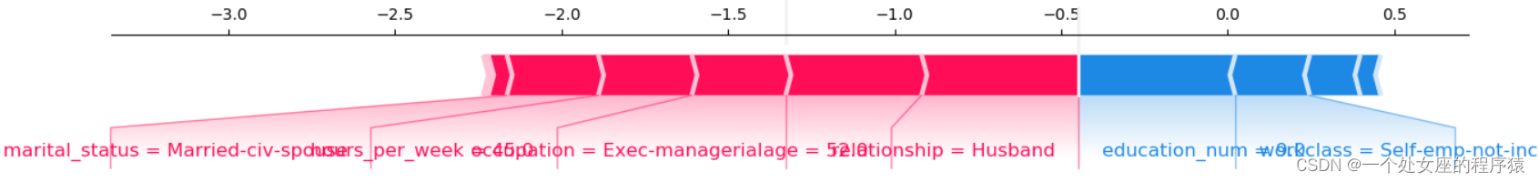
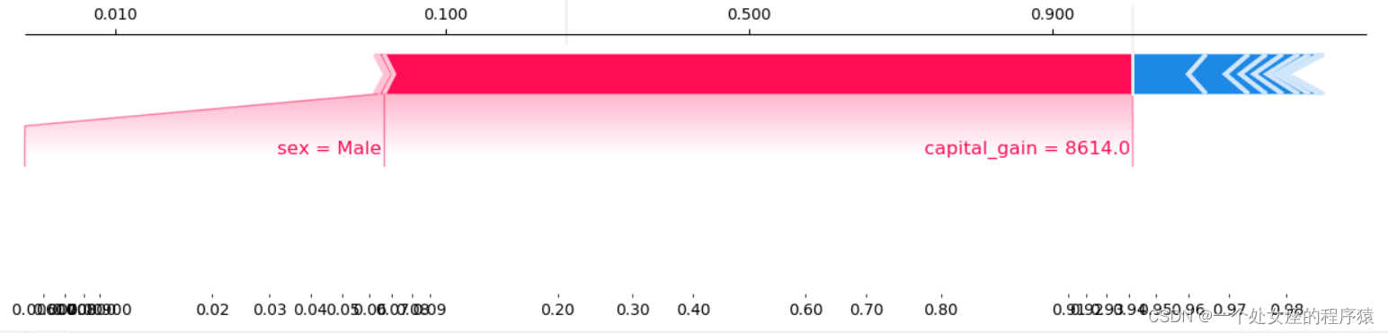
提供了单一模型预测的可解释性,可用于误差分析,找到对特定实例预测的解释。如样例0所示:
(1)、模型输出值:5.89;
(2)、基值:base value即explainer.expected_value,即模型输出与训练数据的平均值;
(3)、绘图箭头下方数字是此实例的特征值。如Age=39;
(4)、红色则表示该特征的贡献是正数(将预测推高的特征),蓝色表示该特征的贡献是负数(将预测推低的特征)。长度表示影响力;箭头越长,特征对输出的影响(贡献)越大。通过 x 轴上刻度值可以看到影响的减少或增加量。
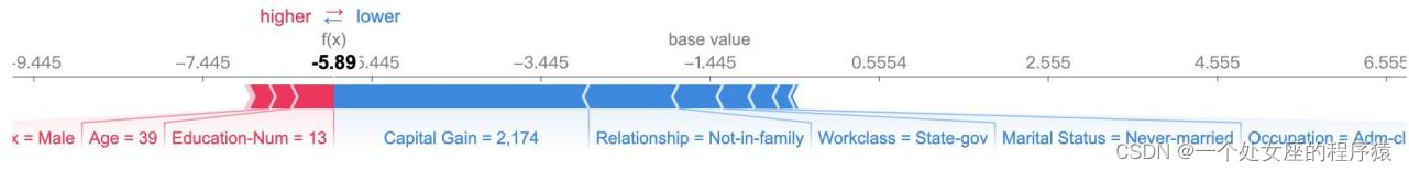
(1)、单个样本力图可视化—对比预测
输出当前测试样本:0

mode_exp_value: -1.3270257
<IPython.core.display.HTML object>
输出当前测试样本:0
 age               29.0
workclass          4.0
education_num      9.0
marital_status     4.0
occupation         1.0
relationship       3.0
race               2.0
sex                0.0
capital_gain       0.0
capital_loss       0.0
hours_per_week    60.0
native_country    39.0
y_val_predi        0.0
y_val              0.0
Name: 11311, dtype: float64
输出当前测试样本的真实label: 0
输出当前测试样本的的预测概率: 0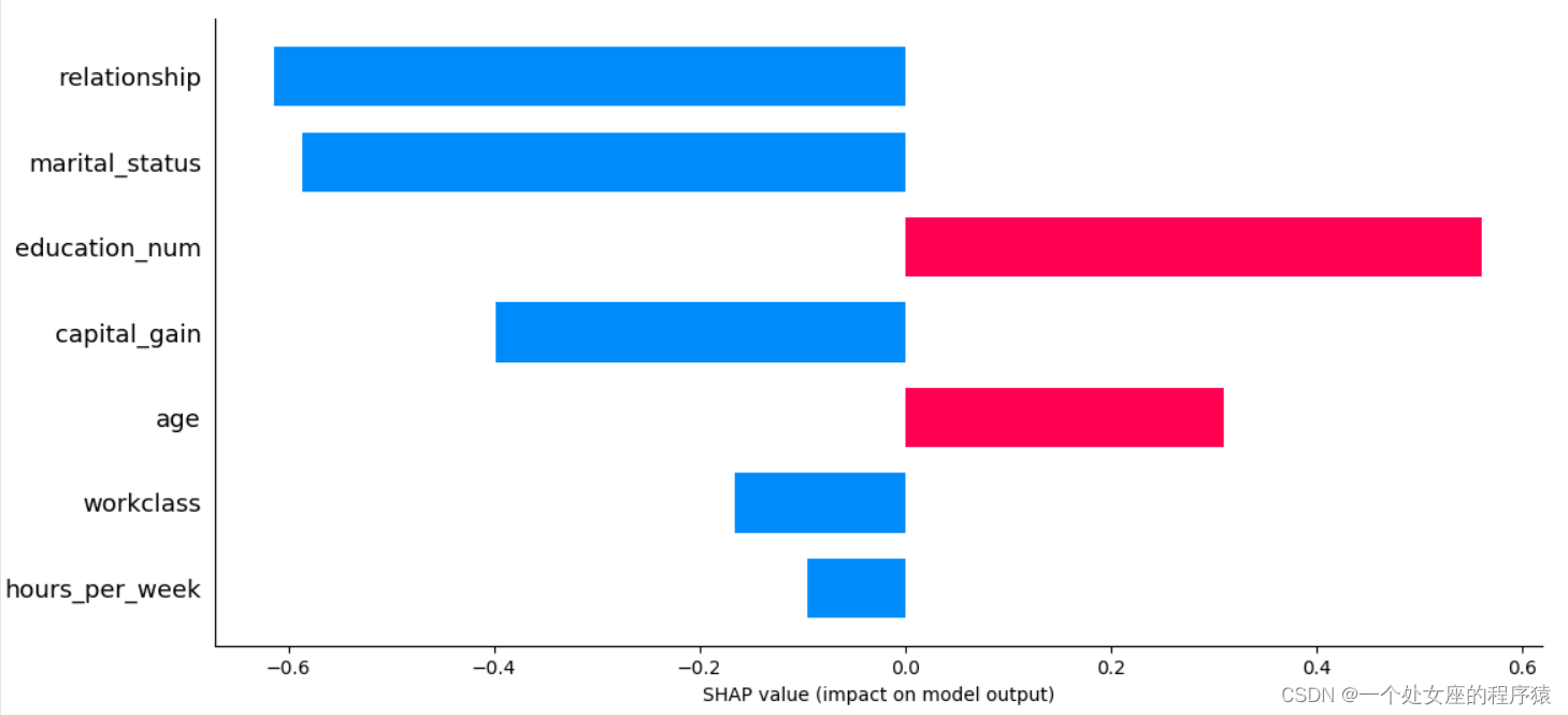
输出当前测试样本:1

输出当前测试样本:1
 age                 33.0
workclass            4.0
education_num       10.0
marital_status       4.0
occupation           3.0
relationship         1.0
race                 2.0
sex                  1.0
capital_gain      8614.0
capital_loss         0.0
hours_per_week      40.0
native_country      39.0
y_val_predi          1.0
y_val                1.0
Name: 12519, dtype: float64
输出当前测试样本的真实label: 1
输出当前测试样本的的预测概率: 1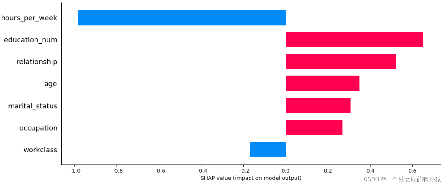
输出当前测试样本:5
输出当前测试样本:5
 age               45.0
workclass          4.0
education_num     10.0
marital_status     2.0
occupation         4.0
relationship       0.0
race               4.0
sex                1.0
capital_gain       0.0
capital_loss       0.0
hours_per_week    40.0
native_country    39.0
y_val_predi        1.0
y_val              0.0
Name: 4319, dtype: float64
输出当前测试样本的真实label: 0
输出当前测试样本的的预测概率: 1
输出当前测试样本:7
输出当前测试样本:7
 age               60.0
workclass          0.0
education_num     13.0
marital_status     2.0
occupation         0.0
relationship       0.0
race               4.0
sex                1.0
capital_gain       0.0
capital_loss       0.0
hours_per_week     8.0
native_country    39.0
y_val_predi        0.0
y_val              1.0
Name: 4721, dtype: float64
输出当前测试样本的真实label: 1
输出当前测试样本的的预测概率: 0
(2)、多个样本力图可视化
# (2.1)、特征贡献度力图可视化,利用深红色深蓝色地图可视化前 5个预测解释,可以使用X数据集。
# (2.2)、误分类力图可视化,肯定要用X_val数据集,因为涉及到模型预测。
如果对多个样本进行解释,将上述形式旋转90度然后水平并排放置,得到力图的变体
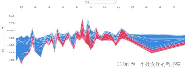
# 5.2、决策图可视化分析:模型如何做出决策
# (1)、单个样本决策图可视化
# (2)、多个样本决策图可视化
# (2.1)、部分样本决策图可视化
# (2.2)、误分类样本决策图可视化
边栏推荐
- How effective is the Chinese-English translation of international economic and trade contracts
- Difference between backtracking and recursion
- LeetCode 739. Daily temperature
- 生物医学英文合同翻译,关于词汇翻译的特点
- 英语论文翻译成中文字数变化
- Wish Dragon Boat Festival is happy
- 云服务器 AccessKey 密钥泄露利用
- Simulation volume leetcode [general] 1061 Arrange the smallest equivalent strings in dictionary order
- LeetCode每日一题(1997. First Day Where You Have Been in All the Rooms)
- Defense (greed), FBI tree (binary tree)
猜你喜欢
The whole process realizes the single sign on function and the solution of "canceltoken" of undefined when the request is canceled

The internationalization of domestic games is inseparable from professional translation companies
![[ 英语 ] 语法重塑 之 英语学习的核心框架 —— 英语兔学习笔记(1)](/img/02/41dcdcc6e8f12d76b9c1ef838af97d.png)
[ 英语 ] 语法重塑 之 英语学习的核心框架 —— 英语兔学习笔记(1)
![[Tera term] black cat takes you to learn TTL script -- serial port automation skill in embedded development](/img/63/dc729d3f483fd6088cfa7b6fb45ccb.png)
[Tera term] black cat takes you to learn TTL script -- serial port automation skill in embedded development

Postman core function analysis - parameterization and test report
基於JEECG-BOOT的list頁面的地址欄參數傳遞

翻译公司证件盖章的价格是多少
Lecture 8: 1602 LCD (Guo Tianxiang)

mysql按照首字母排序

【MQTT从入门到提高系列 | 01】从0到1快速搭建MQTT测试环境
随机推荐
论文摘要翻译,多语言纯人工翻译
红蓝对抗之流量加密(Openssl加密传输、MSF流量加密、CS修改profile进行流量加密)
org.activiti.bpmn.exceptions.XMLException: cvc-complex-type.2.4.a: 发现了以元素 ‘outgoing‘ 开头的无效内容
删除外部表源数据
Simulation volume leetcode [general] 1061 Arrange the smallest equivalent strings in dictionary order
Lesson 7 tensorflow realizes convolutional neural network
On the first day of clock in, click to open a surprise, and the switch statement is explained in detail
Day 248/300 关于毕业生如何找工作的思考
The whole process realizes the single sign on function and the solution of "canceltoken" of undefined when the request is canceled
Summary of leetcode's dynamic programming 4
SSO流程分析
中英对照:You can do this. Best of luck祝你好运
商标翻译有什么特点,如何翻译?
Changes in the number of words in English papers translated into Chinese
Biomedical localization translation services
MFC dynamically creates dialog boxes and changes the size and position of controls
JDBC requset corresponding content and function introduction
Luogu p2141 abacus mental arithmetic test
利用快捷方式-LNK-上线CS
Luogu p2089 roast chicken