当前位置:网站首页>I-BERT
I-BERT
2022-07-06 08:57:00 【cyz0202】
background
In this paper, ICML2021 I-BERT: Integer-only BERT Quantization
The purpose of this article is to BERT Perform more thorough quantization and integer calculations ;
The author believes that the previous quantitative scheme is not right gelu、softmax These nonlinear operations are quantified ( Here's the picture 1), That is to keep float Type of calculation , Not only affects the computational efficiency , And it cannot be deployed on some chips that only support integer Computing ;
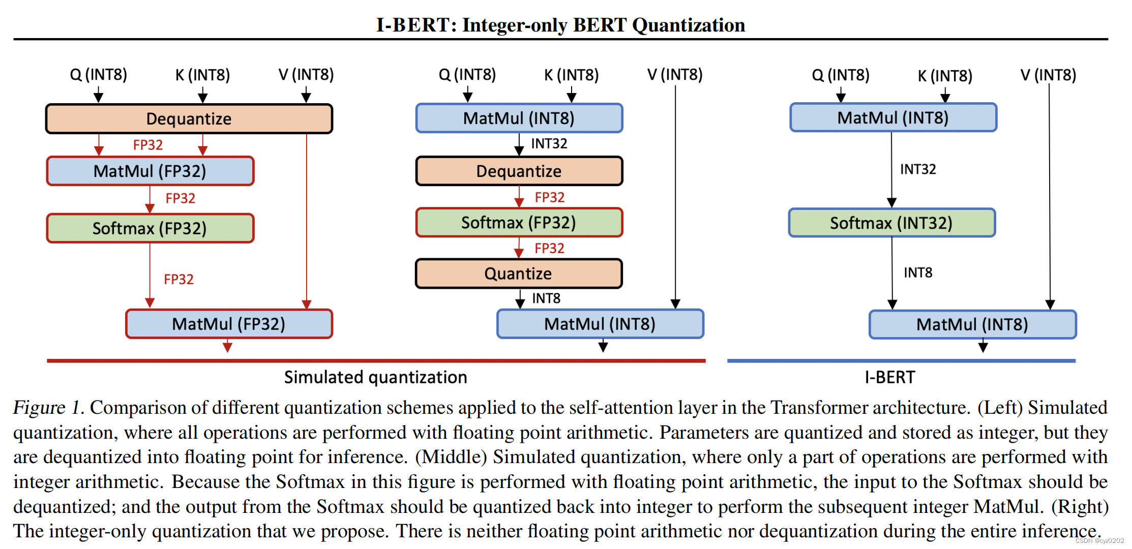
The quantitative scheme adopted by the author is 8bits Symmetric quantization ;
Existing schemes and deficiencies
The author mainly solves GELU、softmax The quantization problem of these two kinds of nonlinear layers ;
First look at it. GELU The expression of , as follows ,erf go by the name of error function
![\\GELU(x) = x*\frac{1}{2}[1+erf(\frac{x}{\sqrt2})]](http://img.inotgo.com/imagesLocal/202207/06/202207060850360827_31.gif)
among ![\\ erf=\frac{2}{\sqrt\pi}\int^x_0e^{-t^2}dt \in [-1, 1] \\](http://img.inotgo.com/imagesLocal/202207/06/202207060850360827_19.gif)
And 
GELU It is difficult to quantify directly , Forced quantization will lead to a large loss of accuracy ;
Unlike linear layers ( Such as matrix product 、 Piecewise linear RELU etc. ), The linear property can be used to inverse quantize to float The result of the calculation is ( The author gives an example MatMul(Sq) = S*MatMul(q), among x=Sq,S by scale,q by x Quantized value of );
Some existing approximations GELU The plan , Include :
- sigmoid The approximate , as follows , Introduce nonlinearity sigmoid, It's still not good for integer calculation

- ReLU6 The approximate , as follows , Use ReLU6, Although it can be integer , But it didn't work ; The program is also known as h-GELU

The figure below 2 The picture on the left shows h-GELU The shortcomings of
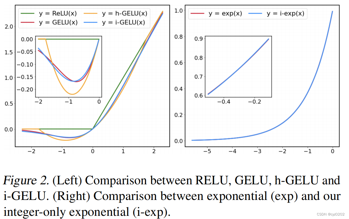
GELU Solutions for
By analyzing , It is considered that second-order polynomial pairs can be introduced erf Make an approximation , Further to GELU Make an approximation , The calculation method is as follows
![\\\underset{a,b,c}{min}\frac{1}{2}||GELU(x) - x*\frac{1}{2}[1+L(\frac{x}{\sqrt2})]||^2_2\\ s.t. \space\ \space\ \space\ L(x) = a(x+b)^2 + c](http://img.inotgo.com/imagesLocal/202207/06/202207060850360827_7.gif)
This idea comes from the theory that any function can be fitted by polynomial function , This type of polynomial is called interpolating polynomials( Interpolation polynomial ); For details, please move to the original ;
The result obtained by directly optimizing the above formula is not ideal , as a result of erf The definition domain of is a real domain scope ;
in consideration of erf The value range of is [-1, 1], And erf It's an odd function , namely

Therefore, the author designs the positive real number field part , And extended to negative real number field , Get the following L(x),
![\\L(x) = sgn(x)*\{a*[clip(|x|, max=-b) + b]^2 + 1\}](http://img.inotgo.com/imagesLocal/202207/06/202207060850360827_29.gif) , among
, among

clip Medium max Express |x| The maximum value is -b;
therefore ![L(x) \in [-1, 1]](http://img.inotgo.com/imagesLocal/202207/06/202207060850360827_14.gif) , And it is an odd function ;
, And it is an odd function ;
a、b By looking for some GELU To solve the fitting problem ;
As can be seen from the above ,
![i-GELU(x) := x*\frac{1}{2}[1 + L(\frac{x}{\sqrt2})]](http://img.inotgo.com/imagesLocal/202207/06/202207060850360827_18.gif)
i-GELU Quantitative scheme of
With GELU Polynomial expression of , You can start designing quantitative solutions ;
L(x) It's a polynomial , So you have to know how to quantize polynomials first ;
The author gives a polynomial Quantization Algorithm I-POLY, as follows
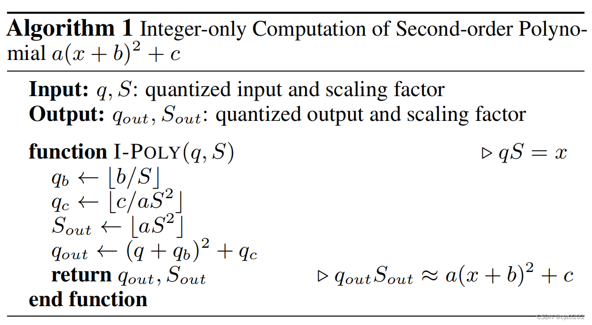
Can verify  ,
,
So arbitrary 2 Quantization of order polynomials 、 The above algorithm can be used for inverse quantization ;
( notes : I feel that the quantification here belongs to a kind of quantification for calculating quantification ; The calculation process is ok , The feeling is deliberately constructed ,q_out and S_out Are not necessarily the real quantized values of polynomial results and scale)
------
With the polynomial quantization method , You can continue to realize I-GELU The quantitative scheme of , The calculation process is as follows
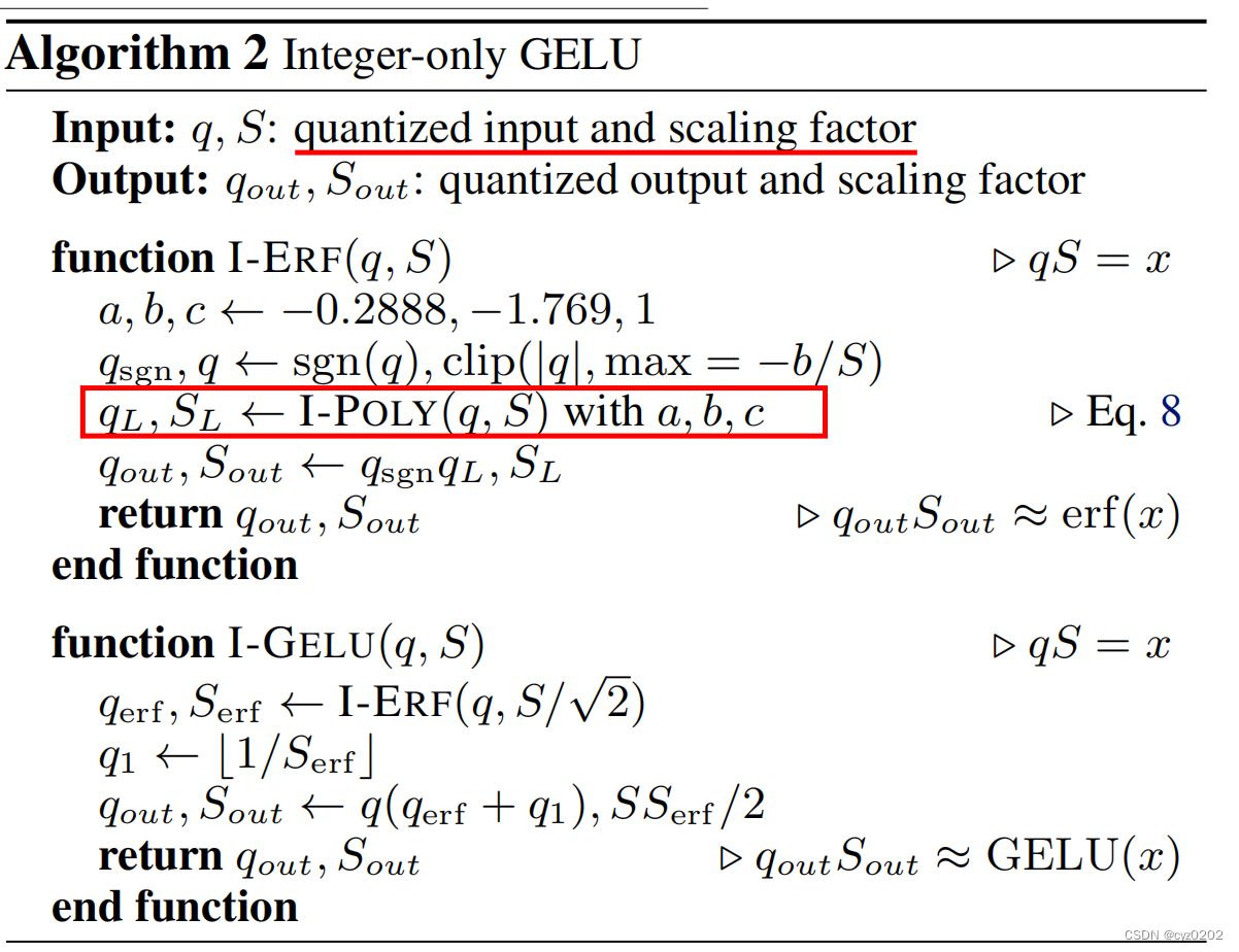
The call stack is I-GELU -> I-ERF -> I-POLY
Pay attention to the picture 4 Some implementation tips in the algorithm , Such as
 ,
,

Notice the above formula max=-b/S, It may have to be changed to max=round(-b/S), Otherwise q’ There is no guarantee that it is integer ...
------
The above is the I-GELU Implementation process , The effect is as follows
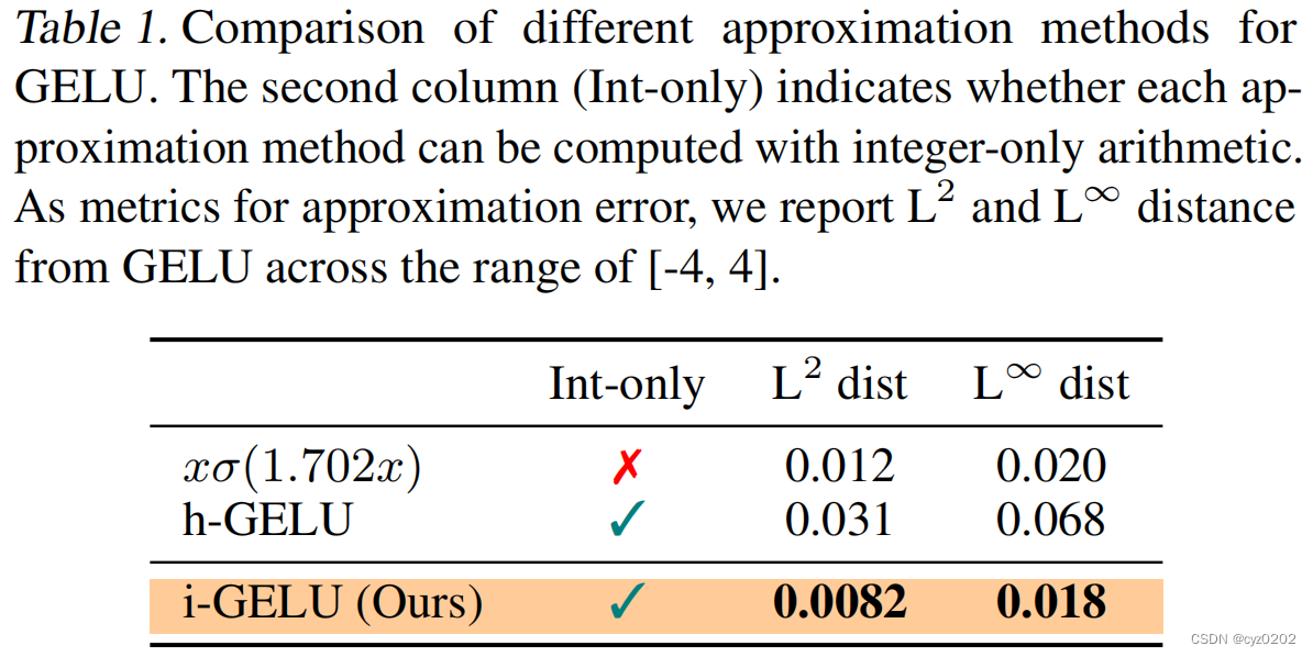
SOFTMAX Solutions for
- Use higher-order polynomials for approximation , Available scenarios are limited ;
SOFTMAX Quantitative scheme of
For numerical stability , The author first gives a brief introduction to softmax To deal with , as follows


It is worth mentioning that ,
For a non positive real number  , It can be approximated by the following formula

among z( merchant ) Is a non negative integer ,p( remainder ) Value range ![(-ln2, 0]](http://img.inotgo.com/imagesLocal/202207/06/202207060850360827_22.gif) ;
;
Then there are

Upper form >> Indicates the right shift operation ;
further , If you can  Expressed as integer calculation , Then it can be used for all
  as well as Softmax Perform integer calculation ;
and  in p Value range of relative x perhaps
  Much smaller , It can be approximated better ;
To recall GELU, The author proposes to adopt 2 Order polynomial approximates nonlinear function ; You can do the same here ;
Author search  The method of approximating second-order polynomials , It is through
 ![(-ln2, 0]](http://img.inotgo.com/imagesLocal/202207/06/202207060850360827_22.gif) Calculate the optimal solution of the following formula in the range :
Calculate the optimal solution of the following formula in the range :

The resulting

be

among  ,
,
chart 2 The figure on the right shows that the above approximation has a good effect ;
Quantitative calculation method of polynomials I-POLY It has been introduced above , So the whole thing Softmax The quantitative calculation method of is
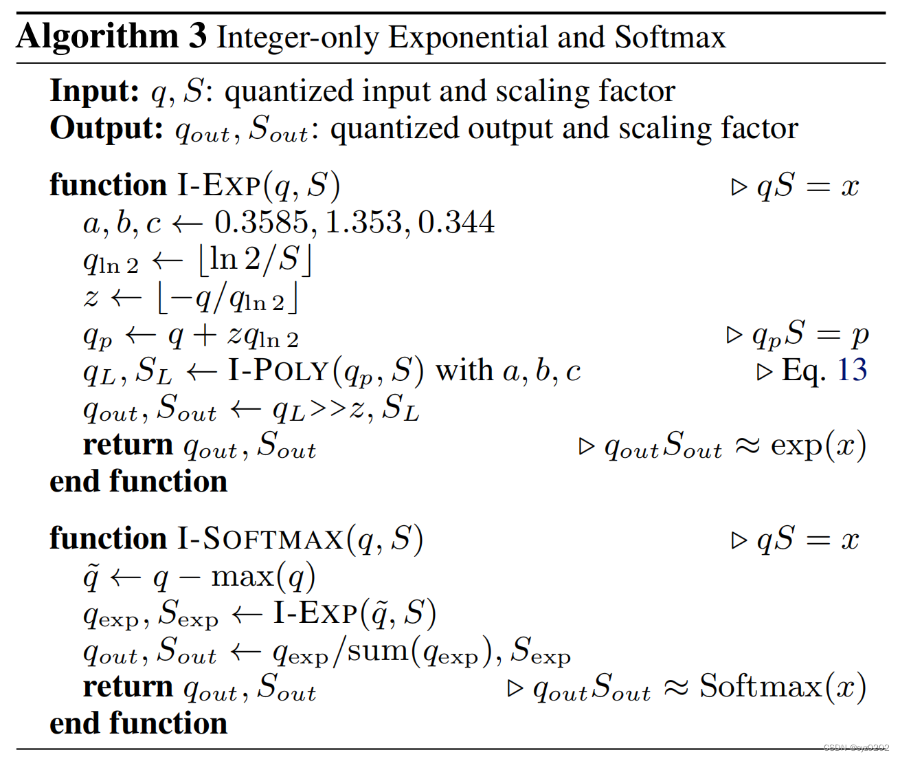
Basic ideas and I-GELU almost
#TODO#: The last step  There seems to be a problem ...
LayerNorm Quantitative scheme of
- To be continued
I-BERT Analysis of the implementation of
- Will be discussed in another article
summary
- This paper introduces I-BERT Improvement points and GELU/SOFTMAX Integer calculation of Implementation method ;
- The main idea is through 2 Order polynomial approximation , Right again 2 Order polynomial for quantitative calculation ;
边栏推荐
- LeetCode:394. 字符串解码
- Hutool gracefully parses URL links and obtains parameters
- Using C language to complete a simple calculator (function pointer array and callback function)
- [OC]-<UI入门>--常用控件-提示对话框 And 等待提示器(圈)
- Simple use of promise in uniapp
- Mise en œuvre de la quantification post - formation du bminf
- LeetCode:34. 在排序数组中查找元素的第一个和最后一个位置
- UML图记忆技巧
- ant-design的走马灯(Carousel)组件在TS(typescript)环境中调用prev以及next方法
- LeetCode:41. 缺失的第一个正数
猜你喜欢
Improved deep embedded clustering with local structure preservation (Idec)

Excellent software testers have these abilities

Ijcai2022 collection of papers (continuously updated)

Navicat premium create MySQL create stored procedure

The ECU of 21 Audi q5l 45tfsi brushes is upgraded to master special adjustment, and the horsepower is safely and stably increased to 305 horsepower
Tcp/ip protocol

Warning in install. packages : package ‘RGtk2’ is not available for this version of R
CUDA实现focal_loss

Cesium draw points, lines, and faces

Alibaba cloud server mining virus solution (practiced)
随机推荐
Show slave status \ read in G_ Master_ Log_ POS and relay_ Log_ The (size) relationship of POS
甘肃旅游产品预订增四倍:“绿马”走红,甘肃博物馆周边民宿一房难求
Intel Distiller工具包-量化实现2
力扣每日一题(二)
[NVIDIA development board] FAQ (updated from time to time)
Esp8266-rtos IOT development
LeetCode:394. String decoding
Leetcode: Jianzhi offer 04 Search in two-dimensional array
MYSQL卸载方法与安装方法
Computer graduation design PHP Zhiduo online learning platform
UnsupportedOperationException异常
Pytorch view tensor memory size
Mise en œuvre de la quantification post - formation du bminf
Advanced Computer Network Review(3)——BBR
Navicat premium create MySQL create stored procedure
LeetCode:剑指 Offer 03. 数组中重复的数字
KDD 2022 paper collection (under continuous update)
LeetCode:214. 最短回文串
UML diagram memory skills
Leetcode: Sword finger offer 48 The longest substring without repeated characters