Using super ball embedding to enhance confrontation training

Use super ball embedding to enhance confrontation training

This is an introduction NeurIPS2020 The job of ,“Boosting Adversarial Training with Hypersphere Embedding”, The first work is from Tsinghua University Tianyu Pang.

This work mainly introduces a technology , be called Hypersphere Embedding, In this paper, it is called hypersphere embedding .

This method is orthogonal to some existing variants of confrontation training , That is, they can integrate with each other to improve the effect .

The variants of confrontation training here are ALP, TRADE etc.

Confrontation training framework

First , As shown in the figure below , Let's list AT And its variants , Mark the differences of their training goals with pink

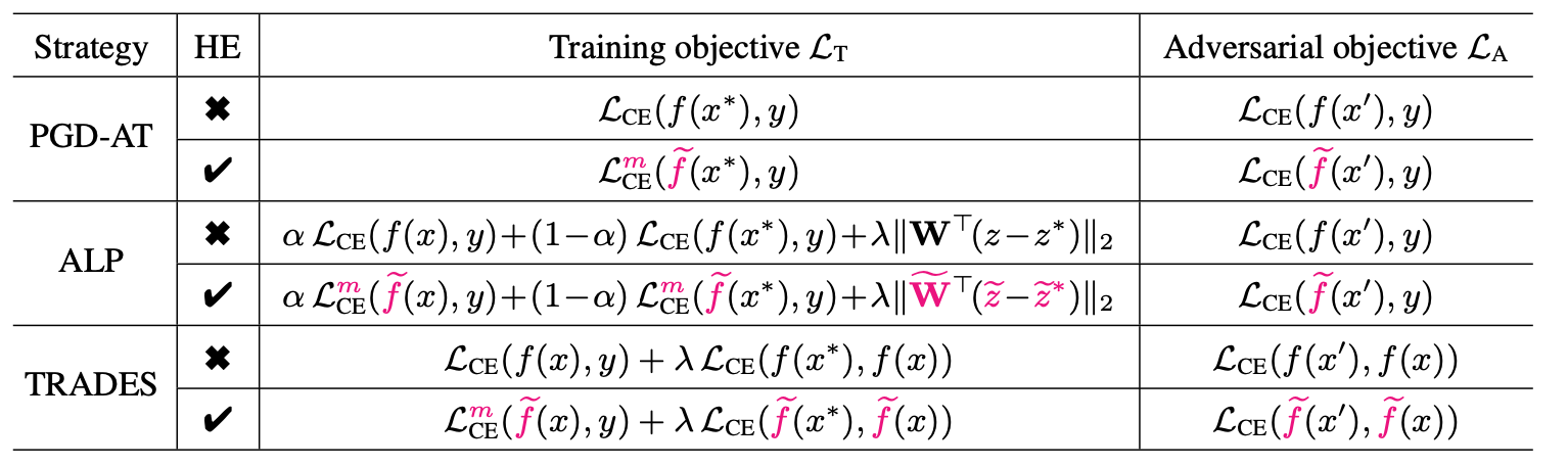
among ,$x^{\ast }$ It's a countermeasure sample , The countermeasure target on the right can be understood as the error function used to generate countermeasure samples .

We can simply see the design of these variants ：

• ALP Is the cross entropy error of normal samples , A regularization term is introduced ,$z$ In fact, that is $f(x)$
• TRADES After introducing the cross entropy error of normal samples , The error of the original countermeasure sample is modified , namely , From the original label $y$ Change to the output of normal samples $f(x)$

HE There are two main parts to modify ：

• In the model $f$ above
• In the cross entropy error ${\mathcal{L}}_{CE}$ above

Methods to introduce

Mark description

Here are some basic marks first , Convenient for later description

We consider classification tasks , Note that the number of labels is $L$, Record the model as :
$$f(x)=\mathbb{S}({\mathbf{W}}^{\top }z+b)$$
among ,$z=z(x;\omega )$ Represents based on model parameters $\omega$ Extracted features , matrix $\mathbf{W}=(W_1,...,W_L)$ And bias $b$ It can be understood as the last linear layer , function $\mathbb{S}(\cdot )$ yes softmax function .

We remember that the cross entropy error is ：
$${\mathcal{L}}_{CE}(f(x),y)=-1_y^{\top }\log f(x)$$
among ,$1_y$ It's the label $y$ Of one-hot code , That is to say $y$ The position is 1, The rest are 0.

We use $\angle (u,v)$ It's a vector $u$ and $v$ The Angle between

The fusion HE Confrontation training framework

First , Most of the confrontation training can be written in the following two-stage framework ：
$$\underset{\omega ,\mathbf{W}}{\min }\mathbb{E}[{\mathcal{L}}_T(\omega ,\mathbf{W}|x,x^{\ast },y)],\text{where }{x}^{\ast }=\arg \underset{x^{\prime }\in \mathbf{B}(x)}{\max }{\mathcal{L}}_A(x^{\prime }|x,y,\omega ,\mathbf{W})$$
In fact, that is , Sir, become a confrontation sample , Then optimize the training objectives .

After many iterations ,$\mathbf{W}$ as well as $\omega$ Will gradually converge , In order to improve the performance of this confrontation training , Some work will metric learning Introduce into confrontation learning , However, the calculation cost of these works is relatively high , It will lead to some category bias , It is still fragile under the stronger counter attack .

Related materials ：

• NeurIPS 2019: Metric learning for adversarial robustness.
• IWSBPR 2015: Deep metric learning using triplet network.
• Stronger resistance to attack ：https://github.com/Line290/FeatureAttack

In fact, the motivation Not enough , The reason given is still not strong enough

Next , Give directly HE In the form of , In fact, it's about characteristics $z$ And weight $\mathbf{W}$ Standardize
$${\mathbf{W}}^{\top }z=(W_1^{\top }z,W_2^{\top }z,...,W_L^{\top }z)$$
among $W_i^{\top }z=\Vert W_i\Vert \Vert z\Vert \cos {\theta }_i$,${\theta }_i=\angle (W_i,z)$

We make
$$\widetilde{W_i}=\frac{W_i}{\Vert W_i\Vert },\tilde{z}=\frac{z}{\Vert z\Vert }$$
Thus there are
$$\begin{gathered} \tilde{f}(x)=\mathbb{S}({\tilde{\mathbf{W}}}^{\top }\tilde{z})=\cos \theta \\ \theta =(\cos {\theta }_1,\cos {\theta }_2,...,\cos {\theta }_L) \end{gathered}$$
When calculating the cross entropy function , Introduce a variable $m$, remember ：
$${\mathcal{L}}_{CE}^m(\tilde{f}(x),y)=-1_y^{\top }\log (\mathbb{S}(s\cdot (\cos \theta -m\cdot 1_y)))$$
among $s>0$ It's a coefficient , Used to improve the stability of values during training

This $m$ The introduction of is a reference CVPR2018 An article from ,Cosface: Large margin cosine loss for deep face recognition

The theoretical analysis

First, we define a vector function ${\mathbb{U}}_p$
$${\mathbb{U}}_p(u)=\arg \underset{\Vert v{\Vert }_p\le 1}{\max }{u}^{\top }v,\text{where }{u}^{\top }{\mathbb{U}}_p(u)=\Vert u{\Vert }_q$$
among $\frac{1}{p}+\frac{1}{q}=1$

lemma 1： Given a counter target error function ${\mathcal{L}}_A$, Make $\mathbf{B}(x)=\{x^{\prime }|\Vert x-x^{\prime }{\Vert }_p\le \epsilon \}$, Using the first-order Taylor expansion , Available ${\max }_{x^{\prime }\in \mathbf{B}(x)}{\mathcal{L}}_A(x^{\prime })$ The solution of is $x^{\ast }=x+\epsilon {\mathbb{U}}_p({\nabla }_x{\mathcal{L}}_A)$. further ,${\mathcal{L}}_A(x^{\ast })={\mathcal{L}}_A(x)+\epsilon \Vert {\nabla }_x{\mathcal{L}}_A(x){\Vert }_q$

prove :

You may as well make $x^{\prime }=x+\epsilon v$, among $\Vert v{\Vert }_p\le 1$

thus ,${\mathcal{L}}_A(x^{\prime })={\mathcal{L}}_A(x+\epsilon v)$

stay $x=x-\epsilon v$ We're going to do a Taylor expansion at , obtain ${\mathcal{L}}_A(x+\epsilon v)\approx {\mathcal{L}}_A(x)+\epsilon v^{\top }({\nabla }_x{\mathcal{L}}_A)$

so ${\max }_{x^{\prime }\in \mathbf{B}(x)}{\mathcal{L}}_A(x^{\prime })={\mathcal{L}}_A(x)+\epsilon {\max }_{\Vert v{\Vert }_p\le 1}{v}^{\top }{\nabla }_x{\mathcal{L}}_A(x)$

I need to use ICML2019 First-order Adversarial Vulnerability of Neural Networks and Input Dimension A knot of On , namely ${\max }_{\delta :\Vert \delta {\Vert }_p\le ϵ}|{\partial }_x\mathcal{L}\cdot \delta |=ϵ\Vert {\partial }_x\mathcal{L}{\Vert }_q,\frac{1}{p}+\frac{1}{q}=1$

Through lemma 1, We got the confrontation sample $x^{\prime }$ For the loss function ${\mathcal{L}}_A$ Influence , At the same time $x$ Yes $x^{\prime }$ The direction of .

lemma 2： Make $W_{ij}=W_i-W_j$ Is the difference between the two weights ,$z^{\prime }=z(x^{\prime };\omega )$ by $x^{\prime }$ Eigenvector of , Then there is
$${\nabla }_{x^{\prime }}{\mathcal{L}}_{CE}(f(x^{\prime }),f(x))=-\sum _{i\ne j}f(x{)}_{i}f(x^{\prime }{)}_j{\nabla }_{x^{\prime }}(W_{ij}^{\top }{z}^{\prime })$$
prove :

$$\begin{array}{rl}-{\nabla }_{x^{\prime }}{\mathcal{L}}_{CE}(f(x^{\prime }),f(x))& ={\nabla }_{x^{\prime }}(f(x{)}^{\top }\log f(x^{\prime }))\\ & =\sum _{i\in [L]}f(x{)}_i{\nabla }_{x^{\prime }}(\log f(x^{\prime }{)}_i)\\ & =\sum _{i\in [L]}f(x{)}_i{\nabla }_{x^{\prime }}(\log [\frac{\exp (W_i^{\top }{z}^{\prime })}{{\sum }_{j\in [L]}\exp (W_j^{\top }{z}^{\prime })}])\\ & =\sum _{i\in [L]}f(x{)}_i{\nabla }_{x^{\prime }}(W_i^{\top }{z}^{\prime }-\log (\sum _{j\in [L]}\exp (W_j^{\top }{z}^{\prime })))\\ & =\sum _{i\in [L]}f(x{)}_i({\nabla }_{x^{\prime }}{W}_i^{\top }{z}^{\prime }-{\nabla }_{x^{\prime }}\log (\sum _{j\in [L]}\exp (W_j^{\top }{z}^{\prime })))\\ & =\sum _{i\in [L]}f(x{)}_i({\nabla }_{x^{\prime }}{W}_i^{\top }{z}^{\prime }-\frac{1}{{\sum }_{j\in [L]}\exp (W_j^{\top }{z}^{\prime })}{\nabla }_{x^{\prime }}(\sum _{j\in [L]}\exp (W_j^{\top }{z}^{\prime })))\\ & =\sum _{i\in [L]}f(x{)}_i({\nabla }_{x^{\prime }}{W}_i^{\top }{z}^{\prime }-\frac{1}{{\sum }_{j\in [L]}\exp (W_j^{\top }{z}^{\prime })}(\sum _{j\in [L]}\exp (W_j^{\top }{z}^{\prime }){\nabla }_{x^{\prime }}(W_j^{\top }{z}^{\prime })))\\ & =\sum _{i\in [L]}f(x{)}_i({\nabla }_{x^{\prime }}{W}_i^{\top }{z}^{\prime }-\sum _{j\in [L]}f(x^{\prime }{)}_j{\nabla }_{x^{\prime }}(W_j^{\top }{z}^{\prime }))\\ & =\sum _{i\in [L]}f(x{)}_i((1-f(x^{\prime }{)}_i){\nabla }_{x^{\prime }}{W}_i^{\top }{z}^{\prime }-\sum _{j\ne i}f(x^{\prime }{)}_j{\nabla }_{x^{\prime }}(W_j^{\top }{z}^{\prime }))\\ & =\sum _{i\in [L]}f(x{)}_i((\frac{{\sum }_{i\ne j}\exp (W_j^{\top }{z}^{\prime })}{{\sum }_{t\in [L]}\exp (W_t^{\top }{z}^{\prime })}){\nabla }_{x^{\prime }}{W}_i^{\top }{z}^{\prime }-\sum _{j\ne i}f(x^{\prime }{)}_j{\nabla }_{x^{\prime }}(W_j^{\top }{z}^{\prime }))\\ & =\sum _{i\in [L]}f(x{)}_i((\frac{{\sum }_{i\ne j}\exp (W_j^{\top }{z}^{\prime })}{{\sum }_{t\in [L]}\exp (W_t^{\top }{z}^{\prime })}){\nabla }_{x^{\prime }}{W}_i^{\top }{z}^{\prime }-\sum _{j\ne i}\frac{\exp (W_j^{\top }{z}^{\prime })}{{\sum }_{t\in [L]}\exp (W_t^{\top }{z}^{\prime })}{\nabla }_{x^{\prime }}(W_j^{\top }{z}^{\prime }))\\ & =\sum _{i\in [L]}f(x{)}_i(\sum _{i\ne j}f(x^{\prime }{)}_j{\nabla }_{x^{\prime }}(W_{ij}^{\top }{z}^{\prime }))\\ & =\sum _{i\ne j}f(x{)}_{i}f(x^{\prime }{)}_j{\nabla }_{x^{\prime }}(W_{ij}^{\top }{z}^{\prime })\end{array}$$

In lemma 2 above , remember $y^{\ast }$ It's a countermeasure sample $x^{\ast }$ Prediction output of , among $y\ne y^{\ast }$

Based on some prior observations , Usually, the probability value of the output tag is predicted （Top1 Probability ） It is much larger than the probability value of other tags

So there is
$${\nabla }_{x^{\prime }}{\mathcal{L}}_{CE}(f(x^{\prime }),f(x))\approx -f(x{)}_{y}f(x^{\prime }{)}_{y^{\ast }}{\nabla }_{x^{\prime }}(W_{y{y}^{\ast }}^{\top }{z}^{\prime })$$
among $W_{y{y}^{\ast }}=W_y-W_{y^{\ast }}$

Make ${\theta }_{y{y}^{\ast }}^{\prime }=\angle (W_{y{y}^{\ast }},z^{\prime })$,$W_{y{y}^{\ast }}^{\top }{z}^{\prime }=\Vert W_{y{y}^{\ast }}\Vert \Vert z^{\prime }\Vert \cos ({\theta }_{y{y}^{\ast }}^{\prime })$ also $W_{y{y}^{\ast }}$ Don't depend on $x^{\prime }$

thus , Iteration of each attack , $x$ The increment of is
$${\mathbb{U}}_p[{\nabla }_{x^{\prime }}{\mathcal{L}}_{CE}(f(x^{\prime }),f(x))]\approx -{\mathbb{U}}_p[{\nabla }_{x^{\prime }}(\Vert z^{\prime }\Vert \cos ({\theta }_{y{y}^{\ast }}^{\prime }))]$$
And the method previously introduced , Will make $\Vert z^{\prime }\Vert =1$, Thus, the attack samples are closer to the classification boundary

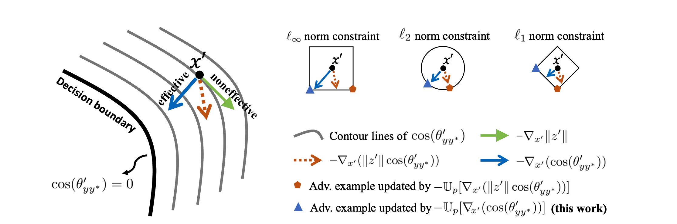
As shown in the figure above ,$\Vert z^{\prime }\Vert$ Will affect the direction of descent , The effect of the generated countermeasure samples is relatively poor , And then inhibit the efficiency of confrontation training

experimental analysis

First of all CIFAR-10 White box attack test on

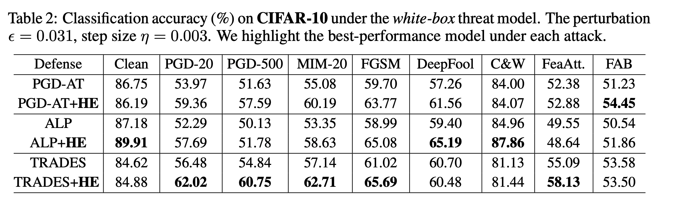
You can see , added HE After that, the defense effect will be improved , In a few cases, it will decline

And then there was ImageNet Test on

comparison FreeAT, The defense effect will be obvious