当前位置:网站首页>[learning notes] matlab self compiled Gaussian smoother +sobel operator derivation
[learning notes] matlab self compiled Gaussian smoother +sobel operator derivation
2022-07-02 07:52:00 【Silent clouds】
This time, we are going to encapsulate the function , Then write the test script
Catalog
Grayscale function encapsulation
Previous notes have written relevant algorithms , Three implementation schemes of grayscale are given . But generally, we don't use loops to traverse , Instead, use slicing . So this time, the packaging grayscale algorithm will become very simple .
stay matlab in , Functions are defined using function. Save the file after writing , It becomes a .m The file of , This is your function file , When calling, it should be placed in the same root directory of your test script , Otherwise, an error will be reported .
% Grayscale function
% The average value is grayed
function result = toGray(img)
    img = double(img);  % The data type of the conversion matrix is double
    gray_img = (img(:,:,1)+img(:,:,2)+img(:,:,3))./3;
    result = uint8(gray_img);
end
./ stay matlab Is used for matrix operation , Every value in the matrix is divided by a number , So the above operation is to extract and add the two-dimensional matrices of the three channels to get a matrix , Then divide all the values in the matrix by 3. and function hinder result Is the output variable , Equivalent to... In other languages return result, It's outgoing result This value . in addition toGray It's the name of the function .
When introducing the grayscale algorithm, I also said ,RGB The image reads out three dimension data , The corresponding difference is : That's ok , Column , dimension .
Encapsulation of convolution function
Or the previous article , Encapsulate the code and it becomes like this :
% Convolution function
function result = myconv(kernel,img)
    [k,num] = size(kernel);
    % Judge whether the incoming is double Data of type , Otherwise, transform
    if ~isa(img,'double')
        p1 = double(img);
    else
        p1 = img;
    end
    [m,n] = size(p1);
    result = zeros(m-k+1,n-k+1);
    for i = ((k-1)/2+1):(m-(k-1)/2)
        for j = ((k-1)/2+1):(n-(k-1)/2)
            result(i-(k-1)/2,j-(k-1)/2) = sum(sum(kernel .* p1(i-(k-1)/2:i+(k-1)/2,j-(k-1)/2:j+(k-1)/2)));
        end
    end
end
Packaging of Gaussian smoother
First, let's introduce Gaussian function , The formula is as follows :
This is a two-dimensional Gaussian distribution function , It is derived from one-dimensional Gaussian function , Then there is nothing then , Anyway, just type the code according to the formula , If you want to know this algorithm in detail , Sure Refer to others Of , It's very detailed .
Now we only need to know the function of Gaussian function . Gauss function , The Gaussian function in one-dimensional form is actually the normal distribution curve of high school , So two important parameters are : One is variance sigma, The other is the coordinates of the curve peak (x Axis ).
Now it's converted to two dimensions , So what you actually draw should be in three-dimensional space , Then the coordinates of the peak become (x0,y0), And the variance is still sigma It hasn't changed .
And the Gaussian smoother in the image , In fact, it is to create a convolution kernel with Gaussian distribution , Then use this convolution kernel to convolute with the original image . This operation is called Gaussian blur .
% Gaussian smoothing filter
function result = gaussian(img,k)
    gray_img = toGray(img); % Image graying
    % Convolution kernel setting
    kernel = zeros(k,k);
    %sigma Determination of size
    %sigma = 0.8;
    sigma = 0.3*((k-1)*0.5-1)+0.8;
    center = 3;
    for i =1:k
        for j = 1:k
            % Gaussian function calculates template parameters
            % Gaussian two-dimensional distribution formula
            temp = exp(-((i-center)^2+(j-center)^2)/(2*sigma^2));
            kernel(i,j) = temp/(2*pi*sigma^2);
        end
    end
    % normalization
    sums = sum(sum(kernel));
    kernel = kernel./sums;
    %
    %
    result = myconv(kernel,gray_img);
end
Parameter description : Among them k Is the size of convolution kernel , It can be 3 It can also be 5 Even larger , The larger the convolution kernel , The higher the blur .
When k=3 when , Its convolution kernel is as follows :
| 0.0009 | 0.0089 | 0.0195 |
|---|---|---|
| 0.0089 | 0.0929 | 0.2030 |
| 0.0195 | 0.2030 | 1.4434 |
Then look at the influence of different convolution kernel sizes on the image .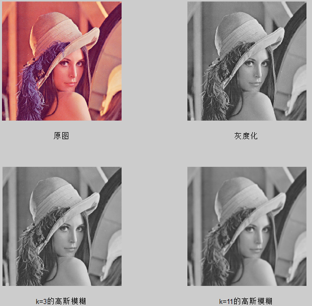
You can see ,k=3 Time has little effect , however k=11 It's obvious when . So what's the use of Gaussian blur ? Why blur the image ? The most important thing is to “ Denoise ”. Because there will be some noise in the image , When doing edge detection , These noises will be treated as edges by mistake , This is not what we hope to see .
utilize Sobel Operator to derive the image
There may be questions here , Why do we need to find the derivative of the image ? And isn't the image actually from a matrix ? So the values are discretized , It doesn't meet the requirements of derivative function at all : Only continuous functions can be derived .
What is the derivative ? What you get is actually the slope of the function . And in the image , What are the characteristics of the edge ? Is the sudden change of gray value . Therefore, the derivative can well describe the change of gray value , Therefore, we can use image derivation to detect edges . Of course , This method is very rough .
Because the image is a bunch of discrete values , So there is no way to use the derivative function to derive the image , That's why there are these “ operator ” The existence of .Sobel The way to derive an operator is to use a 3x3 Convolution kernel to detect , This convolution kernel is divided into x Direction and y The direction of the .
 |  |
% Clean up the previous data
clc;
clear;
% Import image , Or sacrifice our lena Elder sister
img = imread('photo/lena.png');
% Gaussian blur
gray_img = gaossian(img,7);
%sobel operator
x = [1,2,1;0,0,0;-1,-2,-1];
y = [-1,0,1;-2,0,2;-1,0,1];
% Derivative calculation
% The vertical and horizontal derivative results are obtained respectively
gx = myconv(x,gray_img);
gy = myconv(y,gray_img);
G = abs(gx)+abs(gy);
[m,n] = size(G);
% Define a template
bw = zeros(m,n);
% Set threshold
num=50;
for i = 1:m
for j = 1:n
% If the derivative value is higher than a certain threshold, it is regarded as an edge
if (G(i,j)>num)
bw(i,j) = 255;
else
bw(i,j) = 0;
end
end
end
figure();
subplot(221);
imshow(uint8(gx));
subplot(222);
imshow(uint8(gy));
subplot(223);
imshow(uint8(G));
subplot(224);
imshow(uint8(bw));

lena The image of eldest sister looks a little less obvious , Let's change to a more obvious one , This picture of the wall .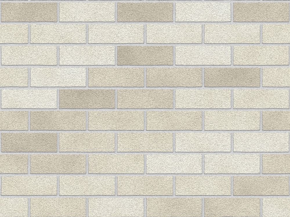

You can see , There is serious noise in this chapter , Just those white dots . If you want to remove , One is to increase the size of Gaussian convolution kernel , The other is to reset the threshold , Raise the threshold .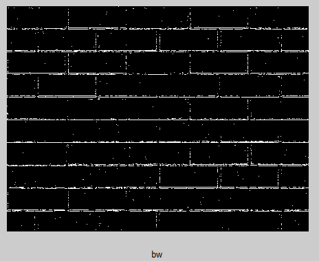
This is to only adjust the threshold to 90 Result , You can see that some edges are missing , But there is still some noise , Now , Other denoising methods can be used for denoising . For example, these white dots belong to salt and pepper noise , Median filtering can be used to remove . Or use corrosion expansion Kit , It's OK to corrode first and then expand .
边栏推荐
- PointNet原理证明与理解
- Correction binoculaire
- Mmdetection trains its own data set -- export coco format of cvat annotation file and related operations
- TimeCLR: A self-supervised contrastive learning framework for univariate time series representation
- 【Sparse-to-Dense】《Sparse-to-Dense:Depth Prediction from Sparse Depth Samples and a Single Image》
- 【Wing Loss】《Wing Loss for Robust Facial Landmark Localisation with Convolutional Neural Networks》
- 【MobileNet V3】《Searching for MobileNetV3》
- 【MagNet】《Progressive Semantic Segmentation》
- 常见的机器学习相关评价指标
- 传统目标检测笔记1__ Viola Jones
猜你喜欢
![[CVPR‘22 Oral2] TAN: Temporal Alignment Networks for Long-term Video](/img/bc/c54f1f12867dc22592cadd5a43df60.png)
[CVPR‘22 Oral2] TAN: Temporal Alignment Networks for Long-term Video

PointNet原理证明与理解

Record of problems in the construction process of IOD and detectron2

label propagation 标签传播
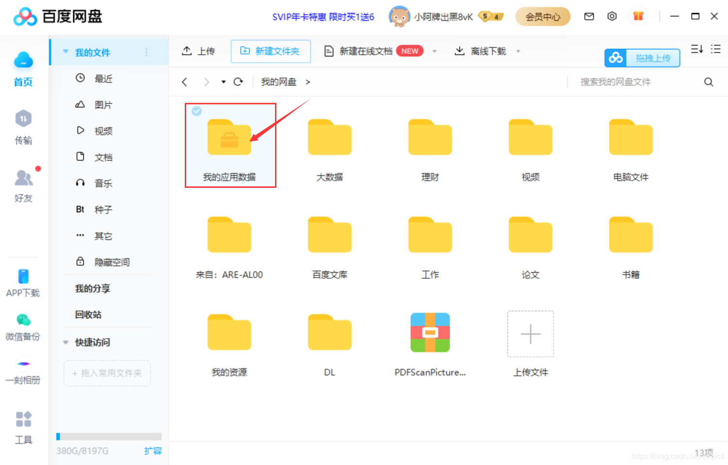
Use Baidu network disk to upload data to the server
How to turn on night mode on laptop
Label propagation
Semi supervised mixpatch

Drawing mechanism of view (I)
Thesis writing tip2
随机推荐
用MLP代替掉Self-Attention
Handwritten call, apply, bind
How to turn on night mode on laptop
联邦学习下的数据逆向攻击 -- GradInversion
【Cascade FPD】《Deep Convolutional Network Cascade for Facial Point Detection》
Common CNN network innovations
【BiSeNet】《BiSeNet:Bilateral Segmentation Network for Real-time Semantic Segmentation》
基于pytorch的YOLOv5单张图片检测实现
【Cutout】《Improved Regularization of Convolutional Neural Networks with Cutout》
【Random Erasing】《Random Erasing Data Augmentation》
Network metering - transport layer
【Cascade FPD】《Deep Convolutional Network Cascade for Facial Point Detection》
MoCO ——Momentum Contrast for Unsupervised Visual Representation Learning
(15) Flick custom source
【Wing Loss】《Wing Loss for Robust Facial Landmark Localisation with Convolutional Neural Networks》
MMDetection安装问题
【深度学习系列(八)】:Transoform原理及实战之原理篇
yolov3训练自己的数据集(MMDetection)
【AutoAugment】《AutoAugment:Learning Augmentation Policies from Data》
【Mixed Pooling】《Mixed Pooling for Convolutional Neural Networks》