当前位置:网站首页>Information and entropy, all you want to know is here
Information and entropy, all you want to know is here
2022-07-05 09:05:00 【aelum】
️ This article references from [d2l] Information Theory
If this article helps you , Can pay attention to ️ + give the thumbs-up + Collection + Leaving a message. , Your support will be the biggest motivation for my creation
Besides , As mentioned in this article log ( ⋅ ) \log(\cdot) log(⋅) Unless otherwise specified, it means log 2 ( ⋅ ) \log_2(\cdot) log2(⋅).
Catalog
One 、 Since the information (Self-information)
Let's start with an example . Roll a dice with even texture , There will be 6 6 6 A possible result , And the probability of each result is 1 / 6 1/6 1/6. Now? :
- Set the event X = { No more than 6 } X=\{\text{ No more than }6\} X={ No more than 6}, Obviously P ( X ) = 1 \mathbb{P}(X)=1 P(X)=1; Besides , This sentence is nonsense , It doesn't tell us anything , Because the number of points you get from rolling a dice will definitely not exceed 6 6 6;
- Set the event X = { No more than 5 } X=\{\text{ No more than }5\} X={ No more than 5}, Obviously P ( X ) = 5 / 6 \mathbb{P}(X)=5/6 P(X)=5/6; Besides , This sentence contains some information , But not much , Because we can almost guess the result ;
- Set the event X = { The number of points is exactly equal to 2 } X=\{\text{ The number of points is exactly equal to }2\} X={ The number of points is exactly equal to 2}, Obviously P ( X ) = 1 / 6 \mathbb{P}(X)=1/6 P(X)=1/6; Besides , This sentence is more informative than the above sentence , because { The number of points is exactly equal to 2 } \{\text{ The number of points is exactly equal to }2\} { The number of points is exactly equal to 2} Contains { No more than 5 } \{\text{ No more than }5\} { No more than 5} Is in there .
As can be seen from this example , An event X X X The amount of information contained is related to the probability of its occurrence . The smaller the probability, the greater the amount of information , The greater the probability, the less information .
Set the event X X X The amount of information contained is I ( X ) I(X) I(X), The probability of its occurrence is p ≜ P ( X ) p\triangleq \mathbb{P}(X) p≜P(X), So how do we find I ( X ) I(X) I(X) And p p p The relationship between ?
First , We have the following common sense :
- Observe a almost The amount of information obtained from certain events almost yes 0 0 0;
- The amount of information obtained by observing two random variables together No more than The amount of information obtained by observing two random variables respectively and , And the inequality is equivalent and only if two random variables Are independent of each other .
Set the event X = { A And B Same as when Hair raw , Its in A 、 B phase mutual single state } X=\{A And B At the same time , among A、B Are independent of each other \} X={ A And B Same as when Hair raw , Its in A、B phase mutual single state }, Obviously P ( X ) = P ( A ) P ( B ) \mathbb{P}(X)=\mathbb{P}(A)\mathbb{P}(B) P(X)=P(A)P(B), And according to the above common sense , And then there is I ( X ) = I ( A ) + I ( B ) I(X)=I(A)+I(B) I(X)=I(A)+I(B). Might as well set I ( ∗ ) = f ( P ( ∗ ) ) I(*)=f(\mathbb{P}(*)) I(∗)=f(P(∗)), be
f ( P ( A ) ⋅ P ( B ) ) = f ( P ( X ) ) = I ( X ) = I ( A ) + I ( B ) = f ( P ( A ) ) + f ( P ( B ) ) f(\mathbb{P}(A)\cdot \mathbb{P}(B))=f(\mathbb{P}(X))=I(X)=I(A)+I(B)=f(\mathbb{P}(A))+f(\mathbb{P}(B)) f(P(A)⋅P(B))=f(P(X))=I(X)=I(A)+I(B)=f(P(A))+f(P(B))
It's not hard to see. log ( ⋅ ) \log(\cdot) log(⋅) Can meet this requirement . But considering that log x \log x logx stay ( 0 , 1 ] (0,1] (0,1] Is non positive and monotonically increasing , So we usually use − log ( ⋅ ) -\log(\cdot) −log(⋅) To measure the amount of information about an event .
Above all , set up event X X X The probability of that happening is zero p p p, The amount of information ( also called Since the information ) It can be calculated in this way :
I ( X ) = − log p (1) \textcolor{red}{I(X)=-\log p\tag{1}} I(X)=−logp(1)
- When ( 1 ) (1) (1) Type in the log \log log With 2 2 2 At the end of the day , The unit of self information is bit \text{bit} bit;
- When ( 1 ) (1) (1) Type in the log \log log With e e e At the end of the day , The unit of self information is nat \text{nat} nat;
- When ( 1 ) (1) (1) Type in the log \log log With 10 10 10 At the end of the day , The unit of self information is hart \text{hart} hart.
You can also get :
1 nat = log 2 e bit ≈ 1.443 bit , 1 hart = log 2 10 bit ≈ 3.322 bit 1\;\text{nat}=\log_2 e\;\text{bit}\approx 1.443 \;\text{bit},\quad 1\;\text{hart}=\log_2 10\;\text{bit}\approx 3.322 \;\text{bit} 1nat=log2ebit≈1.443bit,1hart=log210bit≈3.322bit
We know , For any length of n n n The binary sequence of , It contains n n n Bits of information . for example , For the sequence 0010 0010 0010, The probability of its occurrence is 1 / 2 4 1/2^4 1/24, therefore
I ( “ 0010 ” ) = − log 1 2 4 = 4 bits I(\text{“\,0010\,”})=-\log\frac{1}{2^4}=4\;\text{bits} I(“0010”)=−log241=4bits
Two 、 entropy (Entropy)
set up A random variable X X X Obey the distribution D \mathcal{D} D, be X X X The entropy of is defined as the expectation of its amount of information :
H ( X ) = E X ∼ D [ I ( X ) ] (2) \textcolor{red}{H(X)=\mathbb{E}_{X\sim\mathcal{D}}[I(X)]}\tag{2} H(X)=EX∼D[I(X)](2)
if X X X It's a discrete distribution , be
H ( X ) = − E X ∼ D [ log p i ] = − ∑ i p i log p i H(X)=-\mathbb{E}_{X\sim\mathcal{D}}[\log p_i]=-\sum_ip_i\log p_i H(X)=−EX∼D[logpi]=−i∑pilogpi
if X X X Is a continuous distribution , be
H ( X ) = − E X ∼ D [ log p ( x ) ] = − ∫ p ( x ) log p ( x ) d x H(X)=-\mathbb{E}_{X\sim\mathcal{D}}[\log p(x)]=-\int p(x)\log p(x)\text{d}x H(X)=−EX∼D[logp(x)]=−∫p(x)logp(x)dx
In the discrete case , set up X X X Take only k k k It's worth , Then there are : 0 ≤ H ( X ) ≤ log k 0\leq H(X)\leq \log k 0≤H(X)≤logk.
Different from the amount of information , there X X X It's a random variable, not an event
Take the event as a point , Then the amount of information can be regarded as the information generated by a point , And information entropy represents the average amount of information produced by a series of points
In the following chapters, we will only discuss discrete cases , Formulas in continuous cases can be analogized
2.1 Joint entropy (Joint Entropy)
We already know how to calculate X X X Information entropy of , So how to calculate ( X , Y ) (X,Y) (X,Y) Information entropy of ?
set up ( X , Y ) ∼ D (X,Y)\sim\mathcal{D} (X,Y)∼D, The joint probability distribution is p i j ≜ P ( X = x i , Y = y j ) p_{ij}\triangleq \mathbb{P}(X=x_i,Y=y_j) pij≜P(X=xi,Y=yj), Remember again p i = P ( X = x i ) , p j = P ( Y = y j ) p_i=\mathbb{P}(X=x_i),\,p_j=\mathbb{P}(Y=y_j) pi=P(X=xi),pj=P(Y=yj), According to the definition of information entropy, it is similar
H ( X , Y ) = − ∑ i j p i j log p i j (3) \textcolor{red}{H(X,Y)=-\sum_{ij}p_{ij}\log p_{ij}}\tag{3} H(X,Y)=−ij∑pijlogpij(3)
If X = Y X=Y X=Y, be H ( X , Y ) = H ( X ) = H ( Y ) H(X,Y)=H(X)=H(Y) H(X,Y)=H(X)=H(Y); If X X X and Y Y Y Are independent of each other , be p i j = p i ⋅ p j p_{ij}=p_i\cdot p_j pij=pi⋅pj, , in turn,
H ( X , Y ) = − ∑ i j ( p i ⋅ p j ) ( log p i + log p j ) = − ∑ j p j ∑ i p i log p i − ∑ i p i ∑ j p j log p j = H ( X ) + H ( Y ) H(X,Y)=-\sum_{ij}(p_i\cdot p_j)(\log p_i+\log p_j)=-\sum_j p_j\sum_i p_i\log p_i-\sum_ip_i\sum_jp_j\log p_j=H(X)+H(Y) H(X,Y)=−ij∑(pi⋅pj)(logpi+logpj)=−j∑pji∑pilogpi−i∑pij∑pjlogpj=H(X)+H(Y)
Besides , The following inequality always holds :
H ( X ) , H ( Y ) ≤ H ( X , Y ) ≤ H ( X ) + H ( Y ) H(X),H(Y)\leq H(X,Y)\leq H(X)+H(Y) H(X),H(Y)≤H(X,Y)≤H(X)+H(Y)
2.2 Conditional entropy (Conditional Entropy)
Conditional entropy H ( Y ∣ X ) H(Y|X) H(Y∣X) I have a random variable X X X In the case of random variables Y Y Y uncertainty , Defined as X X X Given the conditions Y Y Y The entropy pair of the conditional probability distribution X X X Mathematical expectation :
H ( Y ∣ X ) = ∑ i p i H ( Y ∣ X = x i ) = ∑ i p i ( − ∑ j p j ∣ i log p j ∣ i ) = − ∑ i j p i j log p j ∣ i (4) H(Y|X)=\sum_i p_iH(Y|X=x_i)=\sum_i p_i \left( -\sum_j p_{j|i}\log p_{j|i}\right)=-\sum_{ij}p_{ij}\log p_{j|i}\tag{4} H(Y∣X)=i∑piH(Y∣X=xi)=i∑pi(−j∑pj∣ilogpj∣i)=−ij∑pijlogpj∣i(4)
utilize p j ∣ i = p i j / p i p_{j|i}=p_{ij}/p_i pj∣i=pij/pi Available
H ( Y ∣ X ) = H ( X , Y ) − H ( X ) H(Y|X)=H(X,Y)-H(X) H(Y∣X)=H(X,Y)−H(X)
It can be seen from the above formula , H ( Y ∣ X ) H(Y|X) H(Y∣X) Actually represents included in Y Y Y But not included in X X X Information in ( Be similar to P ( B \ A ) = P ( A ∪ B ) − P ( A ) \mathbb{P}(B\backslash A)=\mathbb{P}(A\cup B)-\mathbb{P}(A) P(B\A)=P(A∪B)−P(A)).
2.3 Mutual information (Mutual Information)
Given A random variable ( X , Y ) (X,Y) (X,Y), We already know that X X X Information can be used H ( X ) H(X) H(X) To express ; ( X , Y ) (X,Y) (X,Y) The total information can be used H ( X , Y ) H(X,Y) H(X,Y) To express ; Included in Y Y Y But not included in X X X The information in can be used H ( Y ∣ X ) H(Y|X) H(Y∣X) To express . Then what should we measure X X X and Y Y Y All contain information ?
The answer is Mutual information , Its definition is as follows ( It can be understood as a set X X X And Y Y Y Intersection ):
I ( X , Y ) = H ( X , Y ) − H ( Y ∣ X ) − H ( X ∣ Y ) (5) \textcolor{red}{I(X,Y)=H(X,Y)-H(Y|X)-H(X|Y)}\tag{5} I(X,Y)=H(X,Y)−H(Y∣X)−H(X∣Y)(5)
entropy 、 Joint entropy 、 Conditional entropy 、 The relationship between mutual information is as follows :
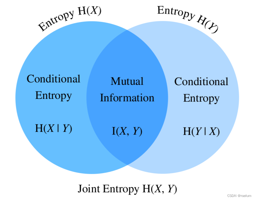
From the above figure, we can also get :
I ( X , Y ) = H ( X ) − H ( X ∣ Y ) I ( X , Y ) = H ( Y ) − H ( Y ∣ X ) I ( X , Y ) = H ( X ) + H ( Y ) − H ( X , Y ) \begin{aligned} I(X,Y)&=H(X)-H(X|Y) \\ I(X,Y)&=H(Y)-H(Y|X) \\ I(X,Y)&=H(X)+H(Y)-H(X,Y) \end{aligned} I(X,Y)I(X,Y)I(X,Y)=H(X)−H(X∣Y)=H(Y)−H(Y∣X)=H(X)+H(Y)−H(X,Y)
We will ( 5 ) (5) (5) Expand the equation to get
I ( X , Y ) = − ∑ i j p i j log p i j + ∑ i j p i j log p j ∣ i + ∑ i j p i j log p i ∣ j = ∑ i j p i j ( log p j ∣ i + log p i ∣ j − log p i j ) = ∑ i j p i j log p i j p i ⋅ p j = E ( X , Y ) ∼ D [ log p i j p i ⋅ p j ] \begin{aligned} I(X,Y)&=-\sum_{ij}p_{ij}\log p_{ij}+\sum_{ij}p_{ij}\log p_{j|i}+\sum_{ij}p_{ij}\log p_{i|j} \\ &=\sum_{ij}p_{ij}(\log p_{j|i}+\log p_{i|j}-\log p_{ij}) \\ &=\sum_{ij} p_{ij} \log \frac{p_{ij}}{p_i\cdot p_j} \\ &=\mathbb{E}_{(X,Y)\sim \mathcal{D}}\left[\log \frac{p_{ij}}{p_i\cdot p_j}\right] \end{aligned} I(X,Y)=−ij∑pijlogpij+ij∑pijlogpj∣i+ij∑pijlogpi∣j=ij∑pij(logpj∣i+logpi∣j−logpij)=ij∑pijlogpi⋅pjpij=E(X,Y)∼D[logpi⋅pjpij]
Some properties of mutual information :
- symmetry : I ( X , Y ) = I ( Y , X ) I(X,Y)=I(Y,X) I(X,Y)=I(Y,X);
- Nonnegativity : I ( X , Y ) ≥ 0 I(X,Y)\geq 0 I(X,Y)≥0;
- I ( X , Y ) = 0 I(X,Y)=0 I(X,Y)=0 ⇔ \;\Leftrightarrow\; ⇔ X X X And Y Y Y Are independent of each other ;
2.4 Point mutual information (Pointwise Mutual Information)
Point mutual information is defined as :
PMI ( x i , y j ) = log p i j p i ⋅ p j (6) \textcolor{red}{\text{PMI}(x_i,y_j)=\log \frac{p_{ij}}{p_i\cdot p_j}} \tag{6} PMI(xi,yj)=logpi⋅pjpij(6)
combination 2.3 section , We will find that the following relationship holds ( For example, information entropy is the expectation of information quantity , Mutual information is also the expectation of point mutual information )
I ( X , Y ) = E ( X , Y ) ∼ D [ PMI ( x i , y j ) ] I(X,Y)=\mathbb{E}_{(X,Y)\sim \mathcal{D}}\left[\text{PMI}(x_i,y_j)\right] I(X,Y)=E(X,Y)∼D[PMI(xi,yj)]
PMI The higher the value of , Express x i x_i xi And y j y_j yj The stronger the correlation .PMI Commonly used in NLP Calculate the correlation between two words in the task , But if the corpus is insufficient , There may be p i j = 0 p_{ij}=0 pij=0 The situation of , This leads to the mutual information of two words − ∞ -\infty −∞, Therefore, a correction is needed :
PPMI ( x i , y j ) = max ( 0 , PMI ( x i , y j ) ) \text{PPMI}(x_i,y_j)=\max(0,\text{PMI}(x_i,y_j)) PPMI(xi,yj)=max(0,PMI(xi,yj))
Aforementioned PPMI Also known as On time mutual information (Positive PMI).
3、 ... and 、 Relative entropy (KL The divergence )
Relative entropy (Relative Entropy) Also known as KL The divergence (Kullback–Leibler divergence), The latter is its more common name .
Set the random variable X X X Obey probability distribution P P P, Now let's try another probability distribution Q Q Q To estimate P P P( hypothesis Y ∼ Q Y\sim Q Y∼Q). remember p i = P ( X = x i ) , q i = P ( Y = x i ) p_i=\mathbb{P}(X=x_i),\,q_i=\mathbb{P}(Y=x_i) pi=P(X=xi),qi=P(Y=xi), be KL Divergence is defined as
D KL ( P ∥ Q ) = E X ∼ P [ log p i q i ] = ∑ i p i log p i q i (7) D_{\text{KL}}(P\Vert Q)=\mathbb{E}_{X\sim P}\left[\log \frac{p_i}{q_i}\right]=\sum_ip_i\log \frac{p_i}{q_i}\tag{7} DKL(P∥Q)=EX∼P[logqipi]=i∑pilogqipi(7)
KL Some properties of divergence :
- Asymmetry : D KL ( P ∥ Q ) ≠ D KL ( Q ∥ P ) D_{\text{KL}}(P\Vert Q)\neq D_{\text{KL}}(Q\Vert P) DKL(P∥Q)=DKL(Q∥P);
- Nonnegativity : D KL ( P ∥ Q ) ≥ 0 D_{\text{KL}}(P\Vert Q)\geq 0 DKL(P∥Q)≥0, The equation holds if and only if P = Q P=Q P=Q;
- If exist x i x_i xi bring p i > 0 , q i = 0 p_i>0,\,q_i=0 pi>0,qi=0, be D KL ( P ∥ Q ) = ∞ D_{\text{KL}}(P\Vert Q) =\infty DKL(P∥Q)=∞.
KL Divergence is used to measure the difference between two probability distributions . If the two distributions are exactly equal , be KL Divergence is 0 0 0. therefore ,KL Divergence can be used as a loss function for multi classification tasks .
because KL Divergence does not satisfy symmetry , Therefore, it is not strictly “ distance ”
Four 、 Cross entropy (Cross-Entropy)
We will ( 7 ) (7) (7) Type disassembly
D KL ( P ∥ Q ) = ∑ i p i log p i − ∑ i p i log q i D_{\text{KL}}(P\Vert Q)=\sum_i p_i\log p_i-\sum_i p_i\log q_i DKL(P∥Q)=i∑pilogpi−i∑pilogqi
If order CE ( P , Q ) = − ∑ i p i log q i \text{CE}(P,Q)=-\sum_i p_i\log q_i CE(P,Q)=−∑ipilogqi, Then the above formula can be written as
D KL ( P ∥ Q ) = CE ( P , Q ) − H ( P ) D_{\text{KL}}(P\Vert Q)=\text{CE}(P,Q)-H(P) DKL(P∥Q)=CE(P,Q)−H(P)
and CE ( P , Q ) \text{CE}(P,Q) CE(P,Q) That's what we're talking about Cross entropy , It is formally defined as
CE ( P , Q ) = − E X ∼ P [ log q i ] (8) \textcolor{red}{\text{CE}(P,Q)=-\mathbb{E}_{X\sim P}[\log q_i]}\tag{8} CE(P,Q)=−EX∼P[logqi](8)
combination KL Nonnegativity of divergence , We can also get CE ( P , Q ) ≥ H ( P ) \text{CE}(P,Q)\geq H(P) CE(P,Q)≥H(P), This inequality is also called Gibbs inequality .
Usually CE ( P , Q ) \text{CE}(P,Q) CE(P,Q) It will also be written as H ( P , Q ) H(P,Q) H(P,Q)
An example of cross entropy calculation :
P P P It's a real distribution , and Q Q Q Is the estimated distribution , Consider the three classification problem , For a sample , The actual labels and predicted results are listed in the following table :
| Category 1 | Category 2 | Category 3 | |
|---|---|---|---|
| target | 0 | 1 | 0 |
| prediction | 0.2 | 0.7 | 0.1 |
As can be seen from the table above , The real situation of this sample belongs to category 2, And p 1 = 0 , p 2 = 1 , p 3 = 0 , q 1 = 0.2 , q 2 = 0.7 , q 3 = 0.1 p_1=0,p_2=1,p_3=0,q_1=0.2,q_2=0.7,q_3=0.1 p1=0,p2=1,p3=0,q1=0.2,q2=0.7,q3=0.1.
therefore
CE ( P , Q ) = − ( 0 ⋅ log 0.2 + 1 ⋅ log 0.7 + 0 ⋅ log 0.1 ) = − log 0.7 ≈ 0.5146 \text{CE}(P,Q)=-(0\cdot \log 0.2+1\cdot \log 0.7+0\cdot \log 0.1)=-\log 0.7\approx 0.5146 CE(P,Q)=−(0⋅log0.2+1⋅log0.7+0⋅log0.1)=−log0.7≈0.5146
When a data set is given , H ( P ) H(P) H(P) It becomes a constant , therefore KL Both divergence and cross entropy can be used as the loss function of multi classification problems . When the real distribution P P P yes One-Hot Vector time , Then there are H ( P ) = 0 H(P)=0 H(P)=0, At this point, the cross entropy is equal to KL The divergence
4.1 Binary cross entropy (Binary Cross-Entropy)
Binary cross entropy (BCE) Is a special case of cross entropy
BCE ( P , Q ) = − ∑ i = 1 2 p i log q i = − ( p 1 log q 1 + p 2 log q 2 ) = − ( p 1 log q 1 + ( 1 − p 1 ) log ( 1 − q 1 ) ) \begin{aligned} \text{BCE}(P,Q)&=-\sum_{i=1}^2p_i\log q_i \\ &=-(p_1\log q_1+p_2\log q_2) \\ &=-(p_1\log q_1+(1-p_1)\log (1-q_1))\qquad \end{aligned} BCE(P,Q)=−i=1∑2pilogqi=−(p1logq1+p2logq2)=−(p1logq1+(1−p1)log(1−q1))
BCE It can be used as the loss function of two classification or multi label classification .
The loss of cross entropy is usually followed by Softmax, The binary cross entropy loss is usually followed by Sigmoid
Under the second category , The output layer can use a neuron +Sigmoid Two neurons can also be used +Softmax, The two are equivalent , But it's faster to train with the former
BCE Can also be through MLE obtain . Given n n n Samples : x 1 , x 2 , ⋯ , x n x_1,x_2,\cdots,x_n x1,x2,⋯,xn, Label of each sample y i y_i yi Not 0 0 0 namely 1 1 1( 1 1 1 Representative positive class , 0 0 0 Representative negative class ), The parameters of neural network are abbreviated as θ \theta θ. Our goal is to find the best θ \theta θ bring y ^ i = P θ ( y i ∣ x i ) \hat{y}_i=\mathbb{P}_{\theta}(y_i|x_i) y^i=Pθ(yi∣xi). set up x i x_i xi The probability of being classified as a positive class is π i = P θ ( y i = 1 ∣ x i ) \pi_i=\mathbb{P}_{\theta}(y_i=1|x_i) πi=Pθ(yi=1∣xi), Then the log likelihood function is
ℓ ( θ ) = log L ( θ ) = log ∏ i = 1 n π i y i ( 1 − π i ) 1 − y i = ∑ i = 1 n y i log π i + ( 1 − y i ) log ( 1 − π i ) \begin{aligned} \ell(\theta)&=\log L(\theta) \\ &=\log \prod_{i=1}^n \pi_i^{y_i}(1-\pi_i)^{1-y_i} \\ &=\sum_{i=1}^ny_i\log \pi_i+(1-y_i)\log (1-\pi_i) \end{aligned} ℓ(θ)=logL(θ)=logi=1∏nπiyi(1−πi)1−yi=i=1∑nyilogπi+(1−yi)log(1−πi)
Maximize ℓ ( θ ) \ell(\theta) ℓ(θ) It's equivalent to minimizing − ℓ ( θ ) -\ell(\theta) −ℓ(θ), The latter is the binary cross entropy loss .
Bloggers lack of talent and knowledge , If there are errors in this article, please point them out in the comment area
边栏推荐
猜你喜欢
Huber Loss
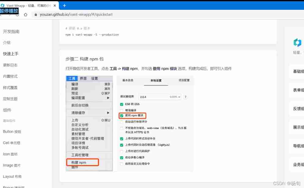
Applet (use of NPM package)
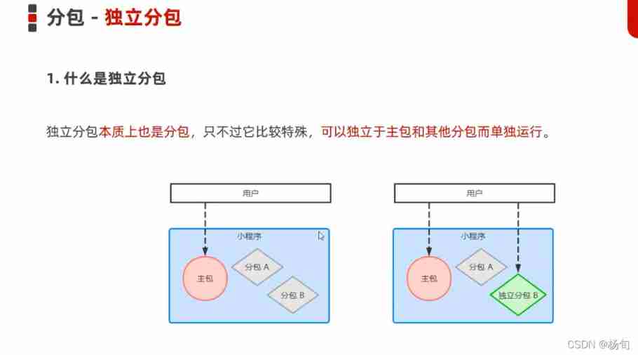
Applet (subcontracting)

Applet (global data sharing)
牛顿迭代法(解非线性方程)
![[daiy4] copy of JZ35 complex linked list](/img/bc/ce90bb3cb6f52605255f1d6d6894b0.png)
[daiy4] copy of JZ35 complex linked list
Solutions of ordinary differential equations (2) examples
![Introduction Guide to stereo vision (4): DLT direct linear transformation of camera calibration [recommended collection]](/img/ed/0483c529db2af5b16b18e43713d1d8.jpg)
Introduction Guide to stereo vision (4): DLT direct linear transformation of camera calibration [recommended collection]
![C [essential skills] use of configurationmanager class (use of file app.config)](/img/8b/e56f87c2d0fbbb1251ec01b99204a1.png)
C [essential skills] use of configurationmanager class (use of file app.config)

Beautiful soup parsing and extracting data
随机推荐
kubeadm系列-01-preflight究竟有多少check
AdaBoost use
Jenkins Pipeline 方法(函数)定义及调用
LLVM之父Chris Lattner:为什么我们要重建AI基础设施软件
[daiy4] copy of JZ35 complex linked list
信息与熵,你想知道的都在这里了
np. allclose
Causes and appropriate analysis of possible errors in seq2seq code of "hands on learning in depth"
520 diamond Championship 7-4 7-7 solution
嗨 FUN 一夏,与 StarRocks 一起玩转 SQL Planner!
golang 基础 —— golang 向 mysql 插入的时间数据和本地时间不一致
Solution to the problem of the 10th Programming Competition (synchronized competition) of Harbin University of technology "Colin Minglun Cup"
我从技术到产品经理的几点体会
Install the CPU version of tensorflow+cuda+cudnn (ultra detailed)
Codeworks round 639 (Div. 2) cute new problem solution
Huber Loss
Rebuild my 3D world [open source] [serialization-3] [comparison between colmap and openmvg]
Transfer learning and domain adaptation
My experience from technology to product manager
Halcon affine transformations to regions