当前位置:网站首页>Chapter VIII integrated learning
Chapter VIII integrated learning
2022-07-08 01:07:00 【Intelligent control and optimization decision Laboratory of Cen】
1. Talk about the concept and thought of integrated learning .
Integrated learning (ensemble learning) Learning tasks are accomplished by building and combining multiple learners , It is sometimes called multi classifier system (multi-classifier system) 、 Committee based learning (committee-based learning) etc. . The schematic diagram of integrated learning is shown below :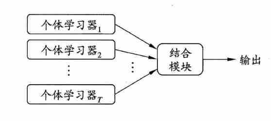
Its main idea is to combine multiple learners , It is often possible to obtain significantly better generalization performance than a single learner . Because the errors of the base learners are independent of each other . In a real task , Individual learners are trained to solve the same problem , They obviously can't be independent of each other ! in fact , Of individual learners " accuracy " and " diversity " There is conflict in itself . General , After high accuracy , Increasing diversity requires sacrificing accuracy . Because the final result is voted by each learner , therefore , How to produce and combine " Good but different " Individual learners of , It is the core of integrated learning research .
2. What kinds of integrated learning methods can be divided into , And explain their characteristics respectively .
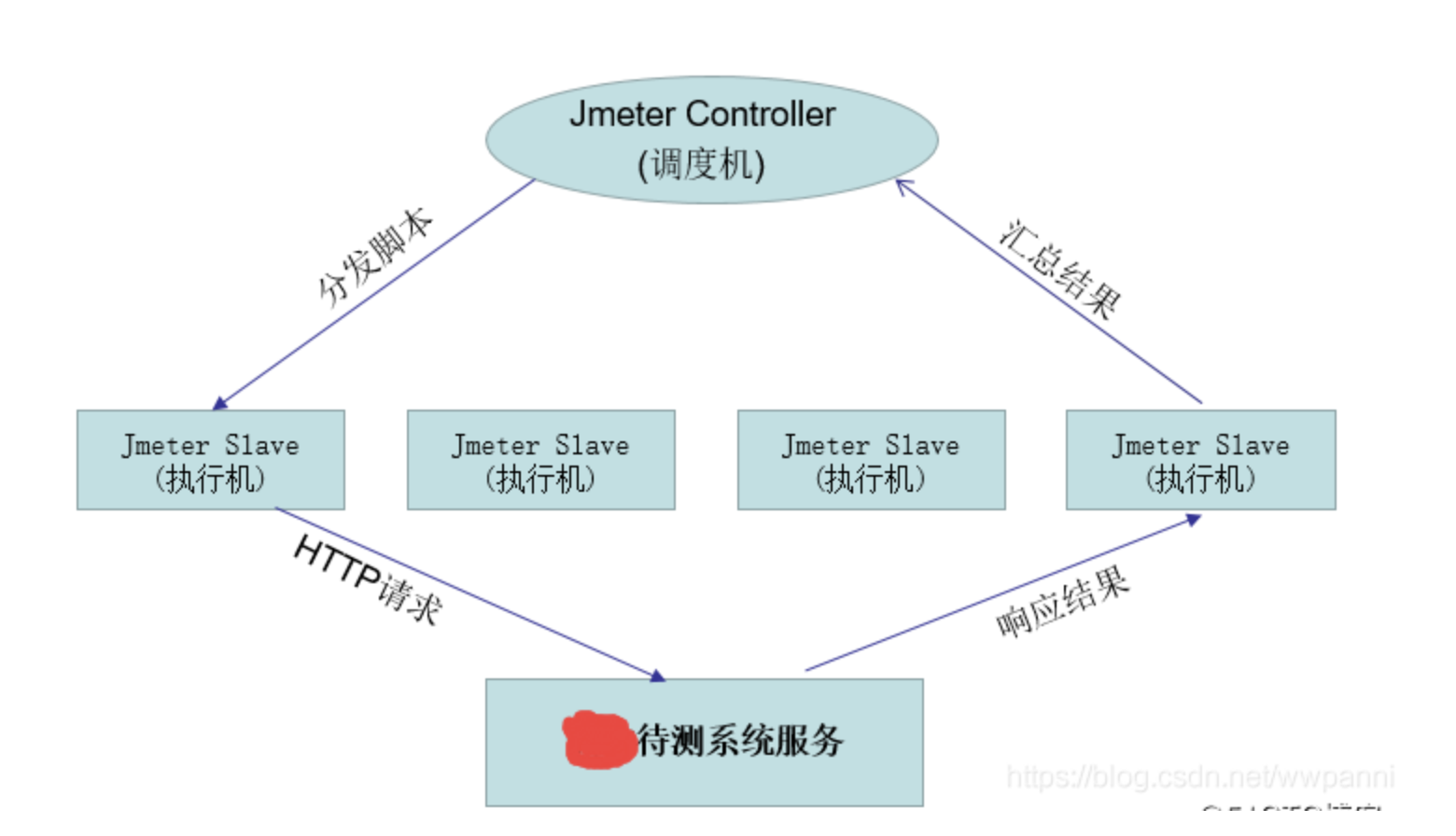
According to how individual learners are generated , The current ensemble learning methods can be roughly divided into two categories ? That is, there is a strong dependency between individual learners 、 Serialization methods that must be generated serially ? And there is no strong dependence between individual learners 、 Parallel methods that can be generated at the same time ; The representative of the former is Boosting, The latter is represented by Bagging and " Random forests " (Random Forest).
- Boosting Method
First, a basic learner is trained from the initial training set , Then adjust the distribution of training samples according to the performance of the basic learner , This makes the training samples that have made mistakes in the previous base learner receive more attention in the follow-up , Then the next base learner is trained based on the adjusted sample distribution ; Repeat it like this , Until the number of base learners reaches a predetermined value T T T, Finally, I will T T T The weighted combination of the base learners is carried out . The flow chart is shown in the figure below :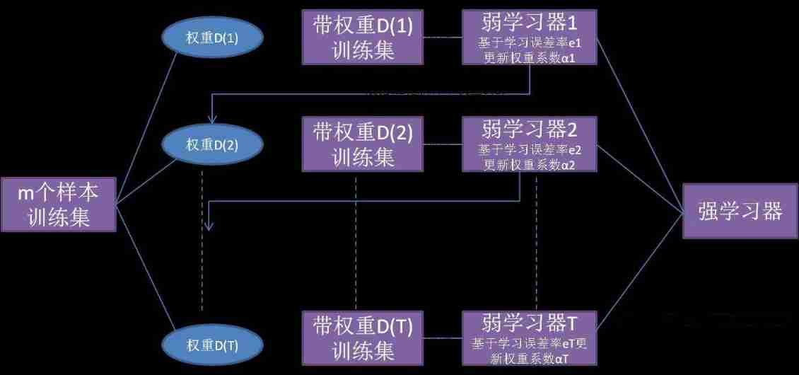
characteristic : Each round of training should check whether the currently generated base learner meets the basic conditions ( Such as whether it is better than random guess ), If the conditions are not met , Then the current learner is discarded , The learning process ends . If the number of study rounds does not reach T T T And lead to poor results , Resampling can be used to restart learning . - Bagging
This kind of method is to sample from the initial training data set T T T Inclusive m m m Sample sets of training samples , Then a base learner is trained based on each sample set , Then combine these basic learning machine roots . The flow chart of this method is shown below :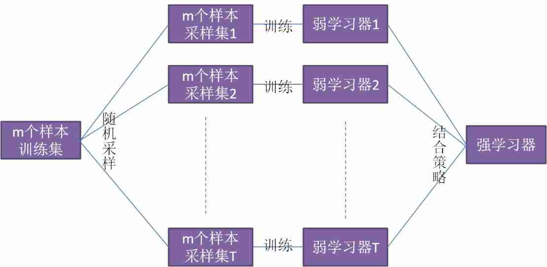
characteristic : Self-help sampling only uses some samples of the initial training set , The remaining samples can be used as validation sets to estimate the generalization performance outside the package ( Pruning can be assisted when the base learner is a decision tree , When the base learner is a neural network , Can reduce the risk of over fitting ).
3. In ensemble learning , Elaborate on the problem of two classifications AdaBoost Algorithm implementation process . reflection AdaBoost How does the algorithm change the weight or probability distribution of the training data in each round ?
3.1 Adaboost Algorithm flow
iterative process :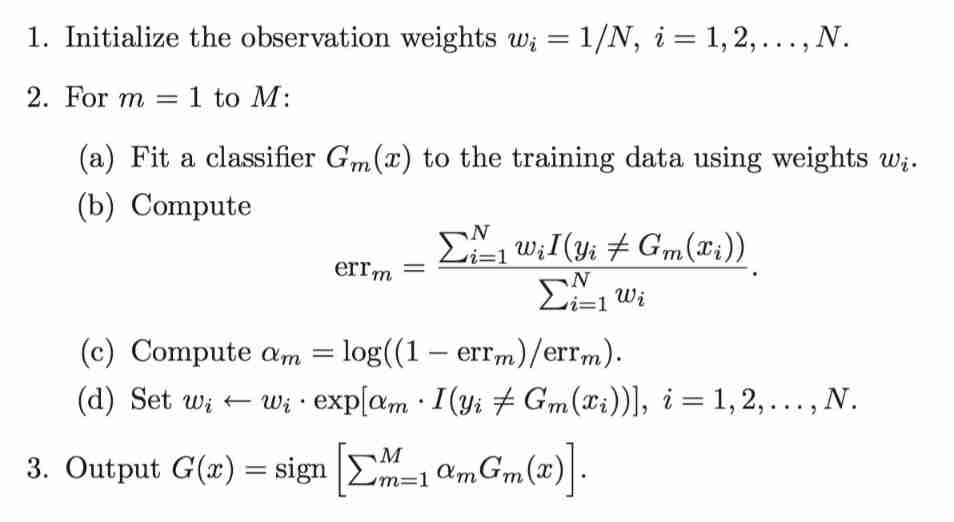
The illustration :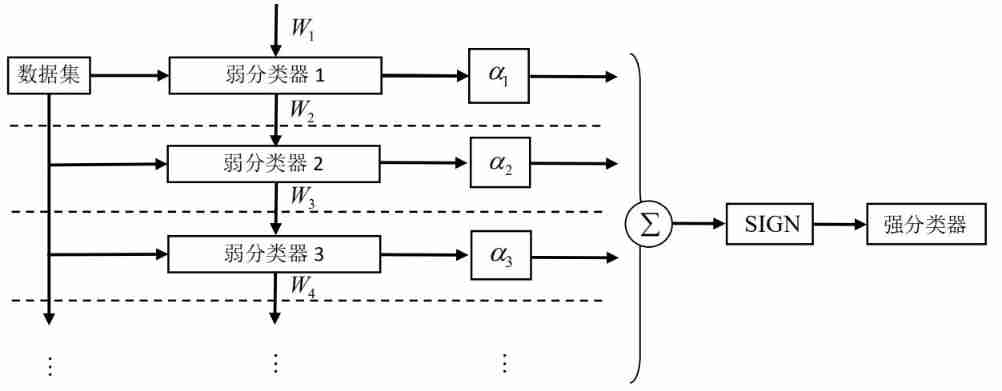
3.2 Main steps :
1. Initialize the weight distribution of training data .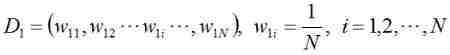
among D 1 D_1 D1 Represents the weight of each sample in the first iteration , w 11 w_{11} w11 Represents the weight of the first sample in the first iteration , N N N Is the total number of samples .
2. Conduct M Sub iteration
a) Use ownership weight distribution D m ( m = 1 , 2 , . . . , N ) D_m(m=1,2,...,N) Dm(m=1,2,...,N) Training samples for learning , Get the weak classifier : G m ( x ) : x → G_m(x):x\rightarrow Gm(x):x→ { − 1 , 1 -1,1 −1,1}.
The performance index of the weak classifier is determined by the value of the following error function ϵ m \epsilon_m ϵm To measure :
b) Compute weak classifiers G m G_m Gm The right to speak α m \alpha_m αm( That is, the weight ), It said G m G_m Gm Importance in final classifier . The calculation method is as follows :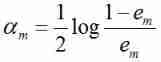
With e m e_m em Reduce , α m \alpha_m αm Gradually increase . The formula shows that , The classifier with small error rate is of great importance in the final classifier .
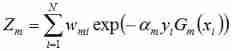
c) Update the weight distribution of training samples , For the next iteration , The weight of the incorrectly classified samples increases , The weight of the correctly classified samples decreases . The calculation method is as follows :

among , D m + 1 D_{m+1} Dm+1 Is the sample value for the next iteration , w m + 1 , 1 w_{m+1,1} wm+1,1 It's the next iteration , The first i i i Weight of samples . y i y_{i} yi On behalf of the i i i Categories corresponding to samples (1 or -1), G m ( x i ) G_m(x_i) Gm(xi) Indicates that the weak classifier pairs samples x i x_{i} xi The classification of . If the classification is correct , be G m ( x i ) G_m(x_i) Gm(xi) The value of is 1, Instead of -1. among Z m ) Z_m) Zm) It's the normalization factor , The calculation method is as follows :
The third step : Combine weak classifiers , Get a strong classifier
First , Weighted sum of all iterated classifiers :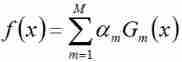
next , take sign The function acts on the sum result , Get the final strong classifier G ( x ) G(x) G(x):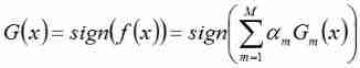
sign function : Is a logical function , The sign used to judge real numbers . The definition for :
4. What is the relationship between random forest and ensemble learning ?
Random forest is an algorithm that integrates multiple trees through the idea of ensemble learning , Its basic unit is the decision tree , And its essence belongs to the integrated learning method .
There are two key words in the name of random forest , One is “ Random ”, One is “ The forest ”.“ The forest ” It's easy for us to understand , One is called a tree , Then hundreds of trees can be called forests , This is also the main idea of random forest – The embodiment of integration thought . However ,bagging The cost of this is not to use a single decision tree to make predictions , Which variable plays an important role becomes unknown , therefore bagging Improved prediction accuracy but lost interpretability .
After learning the decision tree , Understanding the decision tree is simple and intuitive , Easy to understand , The data does not need preprocessing, and the fault tolerance rate for outliers is abnormally high . However, in practice , Decision trees tend to over fit , Unstable performance , This is the need for integration . The theoretical basis is : Law of large Numbers , Under the condition of constant test , Repeat the experiment many times , The frequency of a random event approximates its probability . There is a certain inevitability in contingency .
What is integration ? It's similar to asking thousands of people complicated questions at random , Then summarize their answers , At this time, you will find that their answers are more detailed than those of experts 、 accurate . In machine learning , We all use some estimator to train the model , Now aggregate multiple estimators to Train fitting data , We become integrated learning , This method is called integration method . Random forest is the product of integrated learning , It is composed of a group of decision trees , Each tree is trained based on different two-thirds random subsets in the training set , The growth of each tree is no longer based on the best characteristics , Random forests introduce more randomness into the growth of trees , Instead, select the best feature in a randomly generated feature subset , In this way, the random forest trades higher deviation for lower variance . In this case , Random forests do not have important features like decision trees that appear near heel nodes , Unimportant features appear in leaf nodes unknown . For random forest, we need to calculate the average depth of a feature on all decision trees to estimate The importance of features ( Features can be applied in many ways , For example, whether the credit rating of an enterprise can be correctly evaluated in the bank loan business , It is related to whether the loan can be effectively recovered . But there are many data characteristics of credit evaluation models , There is a lot of noise , So we need to calculate the importance of each feature and rank them , Then we can select the features with high importance from all the features ). This is an important feature of random forest , Apply to feature selection . Finally, as long as we count the results of each tree, we can draw a corresponding conclusion .
5. use python Based on single-layer decision tree AdaBoost Algorithm .
Code :
// An highlighted block
var foo ='bar'';

# -*- coding: utf-8 -*-

import numpy as np

def loadSimData():
    '''
     Input : nothing
     function : Provide a data set with two characteristics
     Output : Datasets with labels
    '''
    datMat = np.matrix([[1. ,2.1],[2. , 1.1],[1.3 ,1.],[1. ,1.],[2. ,1.]])
    classLabels = [1.0, 1.0, -1.0, -1.0, 1.0]
    return datMat, classLabels

def stumpClassify(dataMatrix,dimen,thresholdValue,thresholdIneq):
    '''
     Input : Data matrix , Characteristic dimension , Classification threshold of a feature , Classification inequality
     function : Output decision tree tag
     Output : label
    '''
    returnArray =  np.ones((np.shape(dataMatrix)[0],1))
    if thresholdIneq == 'lt':
        returnArray[dataMatrix[:,dimen] <= thresholdValue] = -1
    else:
        returnArray[dataMatrix[:,dimen] > thresholdValue] = -1
    return returnArray

def buildStump(dataArray,classLabels,D):
    '''
     Input : Data matrix , Corresponding real category label , Weight distribution of features
     function : On the dataset , Find the weighted error rate ( Classification error rate ) The smallest single-layer decision tree , obviously , The index function is closely related to the weight vector
     Output : Best stump ( features , Classification feature threshold , Unequal sign direction ), Minimum weighted error rate , The weight vector D The estimated value of the classification label under
    '''
    dataMatrix = np.mat(dataArray); labelMat = np.mat(classLabels).T
    m,n = np.shape(dataMatrix)
    stepNum = 10.0; bestStump = {
    }; bestClassEst = np.mat(np.zeros((m,1)))
    minError = np.inf
    for i in range(n):
        rangeMin = dataMatrix[:,i].min(); rangeMax = dataMatrix[:,i].max()
        stepSize = (rangeMax - rangeMin)/stepNum
        for j in range(-1, int(stepNum)+1):
            for thresholdIneq in ['lt', 'gt']:
                thresholdValue =  rangeMin + float(j) * stepSize
                predictClass = stumpClassify(dataMatrix,i,thresholdValue,thresholdIneq)
                errArray =  np.mat(np.ones((m,1)))
                errArray[predictClass == labelMat] = 0
                weightError = D.T * errArray
                #print "split: dim %d, thresh: %.2f,threIneq:%s,weghtError %.3F" %(i,thresholdValue,thresholdIneq,weightError)
                if weightError < minError:
                    minError = weightError
                    bestClassEst = predictClass.copy()
                    bestStump['dimen'] = i
                    bestStump['thresholdValue'] = thresholdValue
                    bestStump['thresholdIneq'] = thresholdIneq
    return bestClassEst, minError, bestStump

def adaBoostTrainDS(dataArray,classLabels,numIt=40):
    '''
     Input : Data sets , Label vector , Maximum number of iterations
     function : establish adaboost additive model
     Output : An array of multiple weak classifiers
    '''
    weakClass = []# Define weak classification array , Save each basic classifier bestStump
    m,n = np.shape(dataArray)
    D = np.mat(np.ones((m,1))/m)
    aggClassEst = np.mat(np.zeros((m,1)))
    for i in range(numIt):
        print ("i:",i)
        bestClassEst, minError, bestStump = buildStump(dataArray,classLabels,D)#step1: Find the best single-layer decision tree
        print ("D.T:", D.T)
        alpha = float(0.5*np.log((1-minError)/max(minError,1e-16)))#step2:  to update alpha
        print ("alpha:",alpha)
        bestStump['alpha'] = alpha
        weakClass.append(bestStump)#step3: Add the basic classifier to the array of weak classifiers
        print ("classEst:",bestClassEst)
        expon = np.multiply(-1*alpha*np.mat(classLabels).T,bestClassEst)
        D = np.multiply(D, np.exp(expon))
        D = D/D.sum()#step4: Update weights , This formula is to let D Obey probability distribution
        aggClassEst += alpha*bestClassEst#steo5: Update cumulative category estimates
        print ("aggClassEst:",aggClassEst.T)
        print (np.sign(aggClassEst) != np.mat(classLabels).T)
        aggError = np.multiply(np.sign(aggClassEst) != np.mat(classLabels).T,np.ones((m,1)))
        print ("aggError",aggError)
        aggErrorRate = aggError.sum()/m
        print ("total error:",aggErrorRate)
        if aggErrorRate == 0.0: break
    return weakClass

def adaTestClassify(dataToClassify,weakClass):
    dataMatrix = np.mat(dataToClassify)
    m =np.shape(dataMatrix)[0]
    aggClassEst = np.mat(np.zeros((m,1)))
    for i in range(len(weakClass)):
        classEst = stumpClassify(dataToClassify,weakClass[i]['dimen'],weakClass[i]['thresholdValue']\
                                 ,weakClass[i]['thresholdIneq'])
        aggClassEst += weakClass[i]['alpha'] * classEst
        print (aggClassEst)
    return np.sign(aggClassEst)
if __name__  ==  '__main__':
    D =np.mat(np.ones((5,1))/5)
    dataMatrix ,classLabels= loadSimData()
    bestClassEst, minError, bestStump = buildStump(dataMatrix,classLabels,D)
    weakClass = adaBoostTrainDS(dataMatrix,classLabels,9)
    testClass = adaTestClassify(np.mat([0,0]),weakClass)
result :
// An highlighted block
i: 0
D.T: [[0.2 0.2 0.2 0.2 0.2]]
alpha: 0.6931471805599453
classEst: [[-1.]
 [ 1.]
 [-1.]
 [-1.]
 [ 1.]]
aggClassEst: [[-0.69314718  0.69314718 -0.69314718 -0.69314718  0.69314718]]
[[ True]
 [False]
 [False]
 [False]
 [False]]
aggError [[1.]
 [0.]
 [0.]
 [0.]
 [0.]]
total error: 0.2
i: 1
D.T: [[0.5   0.125 0.125 0.125 0.125]]
alpha: 0.9729550745276565
classEst: [[ 1.]
 [ 1.]
 [-1.]
 [-1.]
 [-1.]]
aggClassEst: [[ 0.27980789  1.66610226 -1.66610226 -1.66610226 -0.27980789]]
[[False]
 [False]
 [False]
 [False]
 [ True]]
aggError [[0.]
 [0.]
 [0.]
 [0.]
 [1.]]
total error: 0.2
i: 2
D.T: [[0.28571429 0.07142857 0.07142857 0.07142857 0.5       ]]
alpha: 0.8958797346140273
classEst: [[1.]
 [1.]
 [1.]
 [1.]
 [1.]]
aggClassEst: [[ 1.17568763  2.56198199 -0.77022252 -0.77022252  0.61607184]]
[[False]
 [False]
 [False]
 [False]
 [False]]
aggError [[0.]
 [0.]
 [0.]
 [0.]
 [0.]]
total error: 0.0
[[-0.69314718]]
[[-1.66610226]]
[[-2.56198199]]
边栏推荐
猜你喜欢
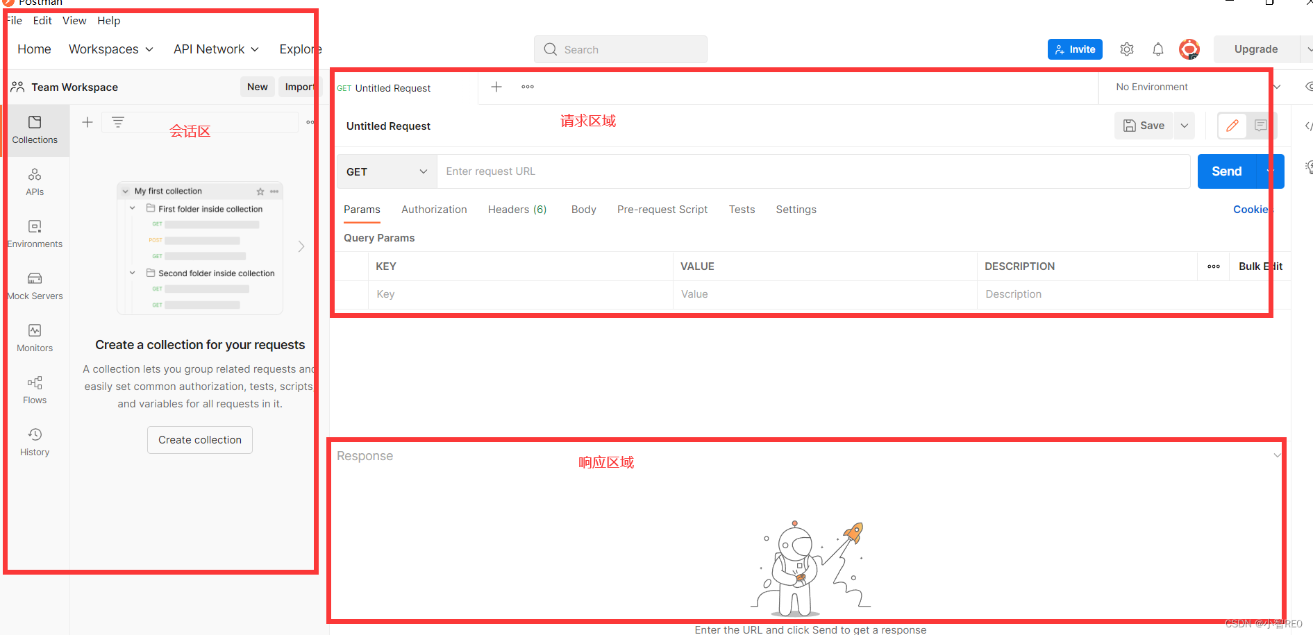
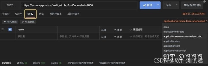
Get started quickly using the local testing tool postman
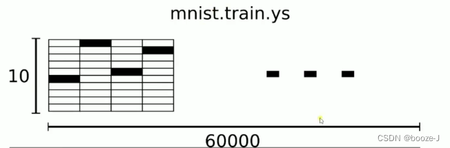
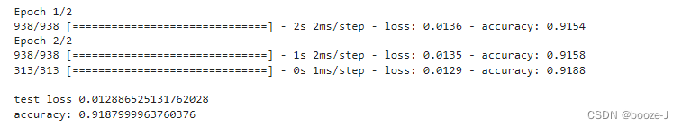
3.MNIST数据集分类
jemter分布式
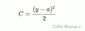
4.交叉熵

Invalid V-for traversal element style
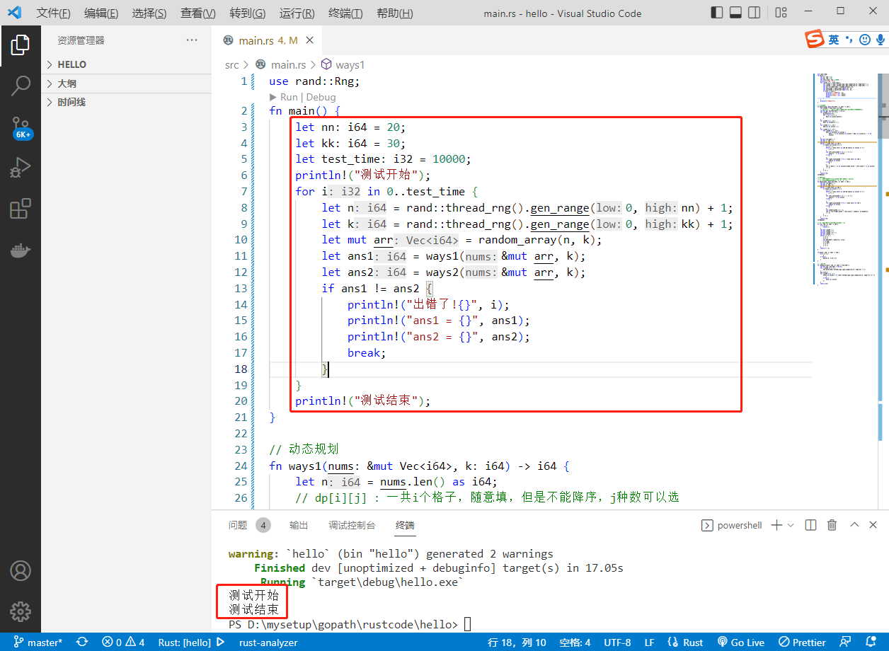
2022-07-07: the original array is a monotonic array with numbers greater than 0 and less than or equal to K. there may be equal numbers in it, and the overall trend is increasing. However, the number
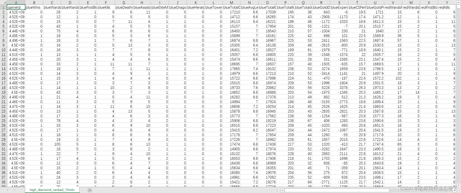
Prediction of the victory or defeat of the League of heroes -- simple KFC Colonel

What has happened from server to cloud hosting?
What does interface testing test?
13.模型的保存和載入
随机推荐
国外众测之密码找回漏洞
Codeforces Round #804 (Div. 2)
Semantic segmentation model base segmentation_ models_ Detailed introduction to pytorch
完整的模型训练套路
2022-07-07: the original array is a monotonic array with numbers greater than 0 and less than or equal to K. there may be equal numbers in it, and the overall trend is increasing. However, the number
Su embedded training - C language programming practice (implementation of address book)
串口接收一包数据
FOFA-攻防挑战记录
Service mesh introduction, istio overview
Cascade-LSTM: A Tree-Structured Neural Classifier for Detecting Misinformation Cascades(KDD20)
12.RNN应用于手写数字识别
letcode43:字符串相乘
Su embedded training - Day9
Cascade-LSTM: A Tree-Structured Neural Classifier for Detecting Misinformation Cascades(KDD20)
Redis, do you understand the list
第四期SFO销毁,Starfish OS如何对SFO价值赋能?
Hotel
新库上线 | CnOpenData中华老字号企业名录
DNS series (I): why does the updated DNS record not take effect?
jemter分布式