当前位置:网站首页>[paper reading] icml2020: can autonomous vehicles identify, recover from, and adapt to distribution shifts?
[paper reading] icml2020: can autonomous vehicles identify, recover from, and adapt to distribution shifts?
2022-07-07 08:24:00 【Kin__ Zhang】
Column: January 6, 2022 7:18 PM
Last edited time: January 30, 2022 12:14 AM
Sensor/ organization : Oxford
Status: Finished
Summary: RIP out-of-distribution, How to consider the phenomenon of uncertainty identification Deal with
Type: ICML
Year: 2020
The amount of citation : 46
In progress → Reference Youtube Better than the paper
References and foreword
Project home page :
PMLR pdf + supplementary pdf:
Can Autonomous Vehicles Identify, Recover From, and Adapt to Distribution Shifts?
github:https://github.com/OATML/oatomobile
arxiv Address :
Can Autonomous Vehicles Identify, Recover From, and Adapt to Distribution Shifts?
youtube ( Advice to see Although it's a little long The comparison Easy to understand ):
1. Motivation
link :out-of-distribution
Deep neural networks usually use Closed world hypothesis Training assumes that the distribution of test data is similar to that of training data . However , When used in real-world tasks , This assumption does not hold , Resulting in a significant decline in their performance .
Why does the model have OOD brittleness ?
- Neural network models may Heavily dependent on training data False clues and annotation artifacts in (spurious cues and annotation artifacts), and OOD The example is unlikely to contain the same false patterns as the examples in the distribution .
- Training data cannot cover all aspects of distribution , Therefore, the generalization ability of the model is limited .
Familiarize yourself with abbreviations :
OOD = out of distribution / Data that does not appear in the training set
RIP = robust imitative planning
Ada RIP = adaptive robust imitative planning
That is, if you encounter a scenario that you did not encounter during training at runtime / data , Although the variance of the model is relatively large , But this information is not used for processing , This paper mainly does :
- When testing the model , distinguish Scenes not encountered in the training set , namely OOD scene
- stay OOD Scene On the model Judge Whether to believe and which one to believe or choice AdaRIP sampling
Problem scenario
[Sugiyama & Kawanabe, 2012; Amodei et al., 2016; Snoek et al., 2019] It has been proved many times , When ML When the model is exposed to a new environment ( That is to say Deviate from the training set In the case of the observed distribution ) when , Because they cannot be generalized , Its reliability will drop sharply , Which leads to disastrous results
give an example : In this picture , Different Model given y 1 , y 3 \mathbf y^1, \mathbf y^3 y1,y3 Is pretty good , But this is because of this scene ( Large disc ) It did not appear in the training set, and the existing model evaluation did not consider completely , Therefore, this paper proposes RIP In this scenario, it will be given for follow path For better y 3 \mathbf y^3 y3, In the figure min k \text{min}_k mink It refers to the same track y i y_i yi Corresponding q1, q2, q3 The smallest
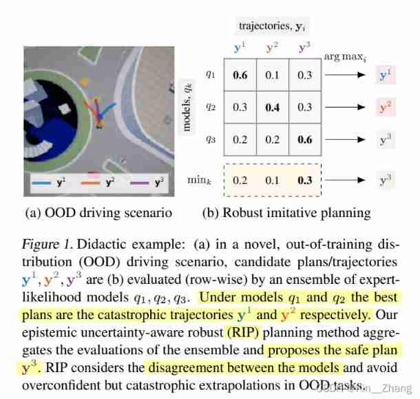
RIP Consider the differences between the models , To avoid the OOD Overconfidence in tasks leads to catastrophic Path result expansion
Although there are other comparisons trick Methods , such as Directly restrict vehicles within the lane line , Based on perception 、e2e Method , But this is also vulnerable spurious correlations. You will also get non causal characteristics And lead to OOD The chaos of actions in the scene
- Dolls about non-causal features that lead to confusion in OOD scenes (de Haan et al., 2019).
In the second half of the introduction, some people's work is cited The existing Baseline But they can't solve this out of distribution problem such as lbc, R2P2
Contribution
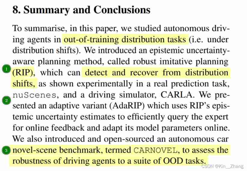
stay conclusion Conclusion There is a concise version in Mainly :formulate out of distribution dataset The uncertainty of , Put forward RIP To solve this uncertain problem makes model robust, One last thing benchmark It is used to make your own model for everyone robust and OOD Performance under the event .
Epistemic uncertainty-aware planning:RIP In fact, it can be regarded as a Simple quantification of epistemic uncertainty with deep ensembles enables detection of distribution shifts.
By using Bayesian decision theory and robust control objectives , Shows how to take conservative actions in unfamiliar situations , This usually enables us to recover from changes in distribution ( Pictured 1)
link :Monte-Carlo Dropout( Monte Carlo dropout),Aleatoric Uncertainty,Epistemic Uncertainty
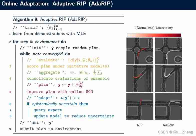
Uncertainty-driven online adaptation: Adaptive robust imitation programming (AdaRIP), Use RIP Cognitive uncertainty estimation to effectively query expert feedback , For immediate adaptation , Without affecting security . therefore ,AdaRIP Can be deployed in the real world : It can reason what it doesn't know , And in these cases Require manual guidance To ensure current security and improve future performance .
Autonomous car novel-scene benchmark: One benchmark be used for Evaluate the robustness of autonomous driving to a set of distributed tasks . Evaluation indicators :
- testing OOD event , Measure by the correlation between violations and model uncertainty
- recover from distribution shift, Quantify by the percentage of successful maneuvers in the new scene
- Adapt effectively OOD scene , Provide online supervision
2. Method
The first is a few assumptions and formula explanation :
Expert data : D = { ( x i , y i ) } i = 1 N \mathcal{D}=\left\{\left(\mathbf{x}^{i}, \mathbf{y}^{i}\right)\right\}_{i=1}^{N} D={ (xi,yi)}i=1N; among , x \mathbf x x It is a high-dimensional observation input , y \mathbf y y yes time-profiled Expert track , So expert strategy expert policy It can be expressed in this way : y ∼ π expert ( ⋅ ∣ x ) \mathbf{y} \sim \pi_{\text {expert }}(\cdot \mid \mathbf{x}) y∼πexpert (⋅∣x)
Imitation learning will be used in the method approximate the unkonwn expert policy
hypothesis Inverse Dynamics: Use PID Conduct Low-level control, This only needs to be aimed at the trajectory y = ( s 1 , ⋯ , s T ) \mathbf y=(s_1,\cdots,s_T) y=(s1,⋯,sT) The action is made by low-level controller To output a t = I ( s t , s t + 1 ) , ∀ t = 1 , … , T − 1 a_{t}=\mathbb{I}\left(s_{t}, s_{t+1}\right), \forall t=1, \ldots, T-1 at=I(st,st+1),∀t=1,…,T−1
Suppose the global planning has , Assume truth location information get
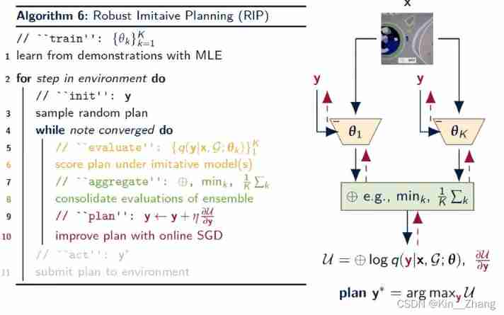
concise : The imitation learning results are expressed by Gaussian probability , Just learn the parameters of the distribution ; And then pass by aggregate and plan Make the final choice
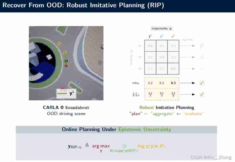
Figure 1 : From link youtube
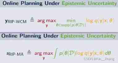
among aggregate step That's the top ⊕ ⊕ ⊕ operator , There are two types shown in the yellow box calculation in Figure 1 :
Take the worst of the strategies Choose the higher of the poor (RIP-WCM) worst case model
Inspired by (Wald,1939)The other is to add all Divide by quantity (RIP-MA) model averaging
Inspired by Bayesian decision theory (Barber, 2012)
There is another kind in the paper RIP-BCM It's found by the author's experience → max k log q k \max_k \log q_k maxklogqk
The formula says
2.1 Expert data
give experts plan Distribution of → Because usually it is a direct action however softmax The previous one should also count distribution Well ?
Bayesian Imitative Model
training via MLE
In the data set D \mathcal{D} D Next distribution density models q ( y ∣ x ; θ ) q(\mathbf y|\mathbf x; \theta) q(y∣x;θ) A posteriori of p ( θ ∣ D ) p(\boldsymbol{\theta}|\mathcal{D}) p(θ∣D) , That is, the model parameters learned first through the data set , Then take it as a priori , Get into probabilisitc imitative mode
θ M L E = arg max θ E ( x , y ) ∼ D [ log q ( y ∣ x ; θ ) ] (1) \boldsymbol{\theta}_{\mathrm{MLE}}=\underset{\boldsymbol{\theta}}{\arg \max } \mathbb{E}_{(\mathbf{x}, \mathbf{y}) \sim \mathcal{D}}[\log q(\mathbf{y} \mid \mathbf{x} ; \boldsymbol{\theta})] \tag{1} θMLE=θargmaxE(x,y)∼D[logq(y∣x;θ)](1)
using probabilisitc imitative model q ( y ∣ x ; θ ) q(\mathbf y|\mathbf x; \theta) q(y∣x;θ); Different from before (Rhinehart et al., 2020; Chen et al., 2019) Here is a prior distribution of model parameters p ( θ ) p(\boldsymbol\theta) p(θ) Used to substitute
Observing x \mathbf x x Next , Experts make y \mathbf y y The probability of is → The author himself said Empirically I found it very effective
q ( y ∣ x ; θ ) = ∏ t = 1 T p ( s t ∣ y < t , x ; θ ) = ∏ t = 1 T N ( s t ; μ ( y < t , x ; θ ) , Σ ( y < t , x ; θ ) ) (2) \begin{aligned}q(\mathbf{y} \mid \mathbf{x} ; \boldsymbol{\theta}) &=\prod_{t=1}^{T} p\left(s_{t} \mid \mathbf{y}_{<t}, \mathbf{x} ; \boldsymbol{\theta}\right) \\&=\prod_{t=1}^{T} \mathcal{N}\left(s_{t} ; \mu\left(\mathbf{y}_{<t}, \mathbf{x} ; \boldsymbol{\theta}\right), \Sigma\left(\mathbf{y}_{<t}, \mathbf{x} ; \boldsymbol{\theta}\right)\right)\end{aligned} \tag{2} q(y∣x;θ)=t=1∏Tp(st∣y<t,x;θ)=t=1∏TN(st;μ(y<t,x;θ),Σ(y<t,x;θ))(2)
among μ ( ⋅ ; θ ) \mu(\cdot ; \boldsymbol \theta) μ(⋅;θ) , Σ ( ⋅ ; θ ) \Sigma(\cdot ; \boldsymbol \theta) Σ(⋅;θ) Are the two RNN, Although the normal distribution is unimodal unimodality , But autoregression ( namely , Future samples depend on the sequential sampling of the past normal distribution ) Allow for multimodal distribution multi-model distribution Modeling
The whole process
- Use deep imitative models As a posterior p ( θ ∣ D ) p(θ|D) p(θ∣D) A simple approximation of
- Consider one K A collection of components , Use θ k θ_k θk To refer to our first k A model q k q_k qk Parameters of
- Through maximum likelihood training ( See formula 1 and Frame diagram b part )
2.2 distinguish OOD
Main comparison posterior p ( θ ∣ D ) p(\boldsymbol{\theta}|\mathcal{D}) p(θ∣D) Under each plan disagreement Use log q ( y ∣ x ; θ ) \log q(\mathbf{y} \mid \mathbf{x} ; \boldsymbol{\theta}) logq(y∣x;θ) The variance of To point out the same policy How different are the different trajectories
u ( y ) ≜ Var p ( θ ∣ D ) [ log q ( y ∣ x ; θ ) ] (3) u(\mathbf{y}) \triangleq \operatorname{Var}_{p(\boldsymbol{\theta} \mid \mathcal{D})}[\log q(\mathbf{y} \mid \mathbf{x} ; \boldsymbol{\theta})]\tag{3} u(y)≜Varp(θ∣D)[logq(y∣x;θ)](3)
Low variance proof in-distribution, The high square difference is OOD
- How to determine this high and low threshold ?
2.3 Post Planning
Alternative planning strategies under cognitive uncertainty ( The red part of the picture below )
Excerpt from youtube in ppt
First formulate Target location under cognitive uncertainty G Planning problems , That is, model parameters p ( θ ∣ D ) p(\boldsymbol{\theta}|\mathcal{D}) p(θ∣D) A posteriori of , Optimization as a general goal (Barber, 2012), We call it robust imitation programming (RIP)
y RIP G ≜ arg max y ⊕ θ ∈ supp ( p ( θ ∣ D ) ) ⏞ aggregation operator log p ( y ∣ G , x ; θ ) ⏟ imitation posterior = arg max y ⊕ θ ∈ supp log q ( y ∣ x ; θ ) ⏟ imitation prior + log p ( G ∣ y ) ⏟ goal likelihood (4) \begin{aligned}\mathbf{y}_{\text {RIP }}^{\mathcal{G}} &\triangleq \underset{\mathbf{y}}{\arg \max } \overbrace{\underset{\boldsymbol{\theta} \in \text { supp }(p(\boldsymbol{\theta} \mid \mathcal{D}))}{\oplus}}^{\text {aggregation operator }} \log \underbrace{p(\mathbf{y} \mid \mathcal{G}, \mathbf{x} ; \boldsymbol{\theta})}_{\text {imitation posterior }} \\&=\underset{\mathbf{y}}{\arg \max } \underset{\boldsymbol{\theta} \in \text { supp }}{\oplus} \log \underbrace{q (\mathbf{y} \mid \mathbf{x} ; \boldsymbol{\theta})}_{\text {imitation prior }}+\log \underbrace{p(\mathcal{G} \mid \mathbf{y})}_{\text {goal likelihood }}\end{aligned}\tag{4} yRIP G≜yargmaxθ∈ supp (p(θ∣D))⊕aggregation operator logimitation posterior p(y∣G,x;θ)=yargmaxθ∈ supp ⊕logimitation prior q(y∣x;θ)+loggoal likelihood p(G∣y)(4)
among ⊕ ⊕ ⊕ Is applied to a posteriori p ( θ ∣ D ) p(\boldsymbol{\theta}|\mathcal{D}) p(θ∣D) The operator of ( See the definition above ), And the target likelihood is determined by, for example, the final target position s T G s^\mathcal{G}_T sTG Gaussian for center and pre specified tolerance p p p give p ( G ∣ y ) = N ( y T ; y T G , ϵ 2 I ) p(\mathcal{G} \mid \mathbf{y})=\mathcal{N}\left(\mathbf{y}_{T} ; \mathbf{y}_{T}^{\mathcal{G}}, \epsilon^{2} I\right) p(G∣y)=N(yT;yTG,ϵ2I)
- It's a bit like Gaussian process Because in the whole T Gaussian process distribution value in time
Just like the formula 4 in plan y R I P G \mathbf y_{RIP}^{G} yRIPG , What we maximize is mainly two parts : From expert data imitation prior, and Close to the final target point G
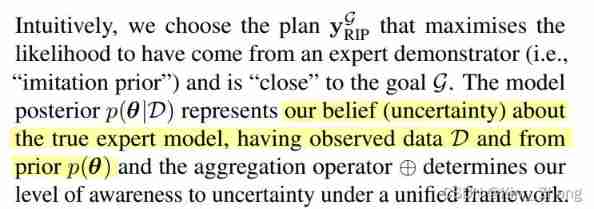
What is pointed out in the original text about posterior p ( θ ∣ D ) p(\boldsymbol{\theta}|\mathcal{D}) p(θ∣D) Yes our belief about the true expert model
emmm But isn't this the model parameter trained through the data set ? Why is a right expert model Of true Probability ? You need to look at the code
It means how much the corresponding model parameters are like this expert plan Do you ? → It's like this
Although the description Deep imitation model DML (Rhinehart et al., 2020) It's a ⊕ ⊕ ⊕ selects a single θ k \theta_k θk from posterior The experiment partially proved So for OOD direct gg
2.4 AdaRIP
can we do better? → Experts step in The blue part
3. experimental result
stay nuScenes: About out-of-distribution How to deal with it ? Do you divide data manually ?
Because in carla in It can be seen that these scenarios are manually selected for testing
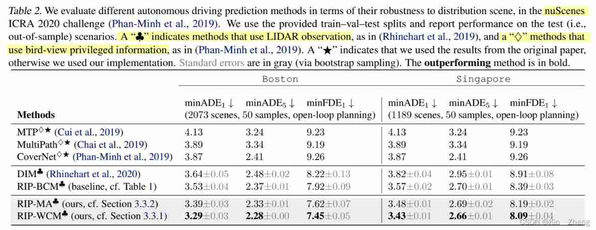
stay nuScenes It's done on the dataset
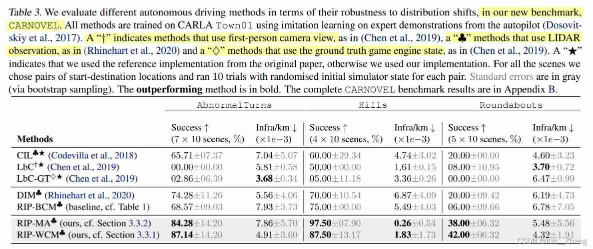
I put forward a benchmark CARNOVEL
4. Conclusion
- Put forward RIP Yes distribution shift Scene recognition and recovery
- AdaRIP Act after understanding the uncertainty , According to online experts feedback Carry out parameter adaptation
- Put forward a benchmark baseline Do this out of distribution problem
Excerpt from the original
This article The author's youtube It's really easier to understand than the paper hhhh ppt It's really good , Each step is also very clear , About open-question I also put forward my own shortcomings in the video ( There are still many deficiencies Mainly involving real vehicles real-time)
- Real time cognitive uncertainty evaluator
- Live online planning
- Resistance to catastrophic forgetting in online adaptation → How to do incremental learning ?
Resistance to catastrophic forgetting in online adaptation
- But I feel that the first real-time method from the paper It can be done , And there is no comparison of time in the full text ? why open question Put forward ? Namely : The experimental part does not explain the real-time effect
Post the code later when you look at the code
- During the group meeting , The little friend pointed out q 1 , q 2 , q 3 q_1, q_2, q_3 q1,q2,q3 If they are all from the same data set , The same training parameters , The model that should be trained is similar , There will be no diversity of choices Pictured 1
- There is also the fact that the theme of this article should be adaptive … But I didn't do it … adapt Artificially , In the words of brothers : It turned out to be adding a layer embedding.
边栏推荐
- Four items that should be included in the management system of integral mall
- Interview questions (CAS)
- 提高企业产品交付效率系列(1)—— 企业应用一键安装和升级
- 漏洞複現-Fastjson 反序列化
- 解析机器人科技发展观对社会研究论
- Rainbond 5.7.1 支持对接多家公有云和集群异常报警
- [go ~ 0 to 1] obtain timestamp, time comparison, time format conversion, sleep and timer on the seventh day
- Uniapp mobile terminal forced update function
- Zcmu--1396: queue problem (2)
- 【雅思口语】安娜口语学习记录 Part2
猜你喜欢
Avatary's livedriver trial experience
Explore creativity in steam art design
Rainbow version 5.6 was released, adding a variety of installation methods and optimizing the topology operation experience
解读创客思维与数学课程的实际运用

Interactive book delivery - signed version of Oracle DBA work notes
Rainbow combines neuvector to practice container safety management
Implement your own dataset using bisenet
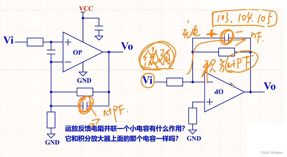
What is the function of paralleling a capacitor on the feedback resistance of the operational amplifier circuit
Unityhub cracking & unity cracking
Battery and motor technology have received great attention, but electric control technology is rarely mentioned?
随机推荐
Openjudge noi 2.1 1752: chicken and rabbit in the same cage
Learn how to compile basic components of rainbow from the source code
Xcit learning notes
PVTV2--Pyramid Vision TransformerV2学习笔记
IP-guard助力能源企业完善终端防泄密措施,保护机密资料安全
[quick start of Digital IC Verification] 12. Introduction to SystemVerilog testbench (svtb)
Using helm to install rainbow in various kubernetes
Snyk 依赖性安全漏洞扫描工具
Pytoch (VI) -- model tuning tricks
The simple problem of leetcode is to judge whether the number count of a number is equal to the value of the number
opencv学习笔记三——图像平滑/去噪处理
CTF-WEB shrine模板注入nmap的基本使用
Don't stop chasing the wind and the moon. Spring mountain is at the end of Pingwu
XCiT学习笔记
buureservewp(2)
提高企业产品交付效率系列(1)—— 企业应用一键安装和升级
The reified keyword in kotlin is used for generics
Opencv learning note 3 - image smoothing / denoising
Avatary's livedriver trial experience
Interview questions (CAS)