当前位置:网站首页>Target detection series - detailed explanation of the principle of fast r-cnn
Target detection series - detailed explanation of the principle of fast r-cnn
2022-07-05 07:13:00 【Bald little Su】
Author's brief introduction : Bald Sue , Committed to describing problems in the most popular language
Looking back : Target detection series —— The work of the mountain RCNN The principle, Target detection series ——Fast R-CNN The principle,
Near term goals : Have 10000 fans
Support Xiao Su : give the thumbs-up 、 Collection 、 Leaving a message.
List of articles
Target detection series ——Faster R-CNN The principle,
Write it at the front
I have already introduced it before R-CNN、Fast R-CNN Principle , Specific content can be read by clicking the link below .【 notes : Before reading this article, I suggest that R-CNN and Fast R-CNN Have some understanding 】
- Target detection series —— The work of the mountain RCNN The principle,
- Target detection series ——Fast R-CNN The principle,
Faster R-CNN It is the last article in this series of target detection , It also achieved relatively good results in speed and accuracy , So it's still very important . Semantic segmentation may be updated later Mask RCNN, Of course, this is all later . Now learn with me Faster R-CNN Well .
Faster R-CNN Overall process
I wonder if you remember Fast R-CNN The process of ? Here to help you recall , The steps are as follows :
- Candidate area generation
- Full image input network , The candidate frame is projected onto the feature graph to obtain the feature matrix
- The characteristic matrix is ROI pooling Layers are scaled to uniform size , Then flatten the characteristic map to get the prediction result
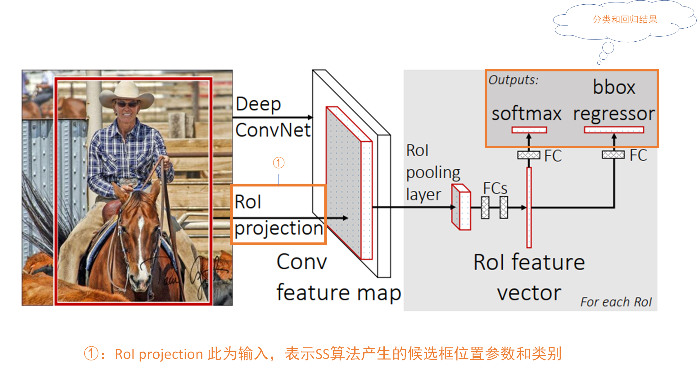
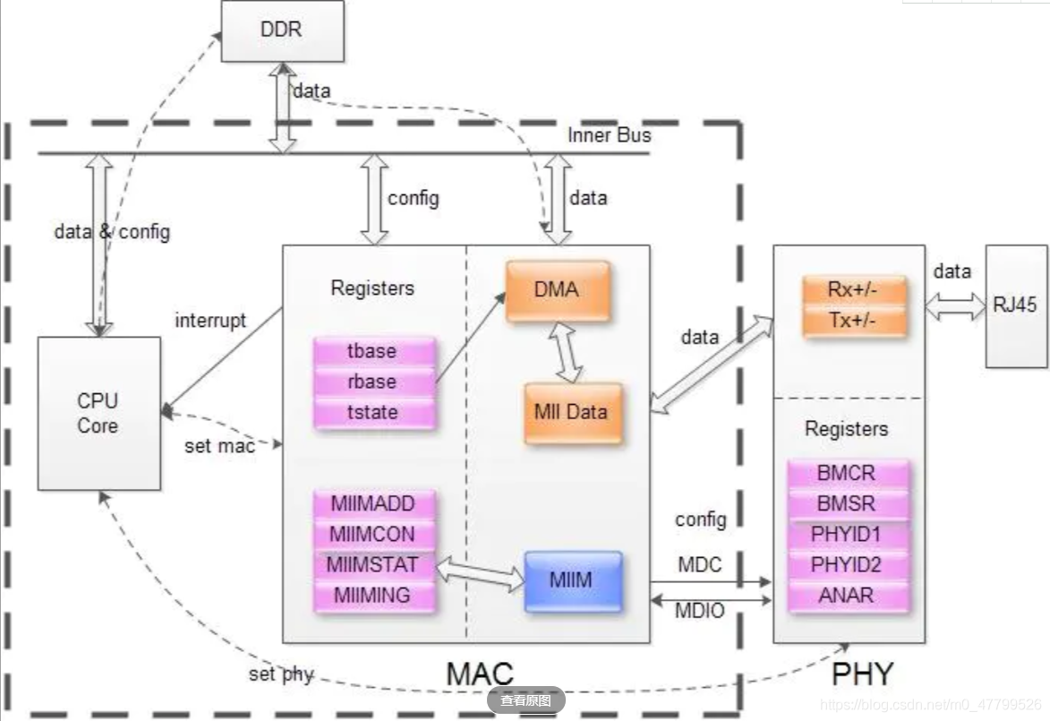
that Faster R-CNN Compare with Fast R-CNN What improvements are needed ? In fact, the most important thing is Fast R-CNN We are still with R-CNN Use the same SS Algorithm to generate candidate box , And in the Faster R-CNN We use a method called RPN(Region Proposal Network) Network structure to generate candidate boxes . Other parts are basically the same as Fast R-CNN Agreement , So we can put Faster R-CNN Our network can be seen as two parts , Part of it is RPN Get the candidate box network structure , The other part is Fast R-CNN Network structure , As shown in the figure below :
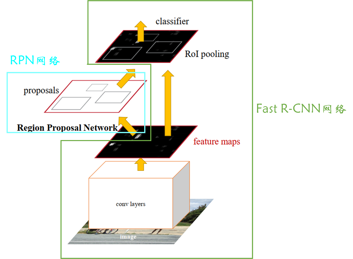
If this is your first time to see Faster R-CNN, Look at this picture , I think you are still in a relatively ignorant state . But it doesn't matter , This figure is given in the paper , The main purpose of my posting here is to let you know roughly Faster R-CNN The structure is good , Then the soul asked —— Do you know the general structure ?
In fact! ,Faster R-CNN The structure and Fast R-CNN It's still very similar , Will produce some candidate boxes , Then, these candidate boxes are classified and regressed based on the feature extraction network , The difference is Fast R-CNN It's traditional SS The algorithm extracts candidate boxes , and Faster R-CNN use RPN Network to extract .
Okay ,Faster R-CNN So much about the overall process , You must still have many doubts , Don't worry , Now let's explain step by step .
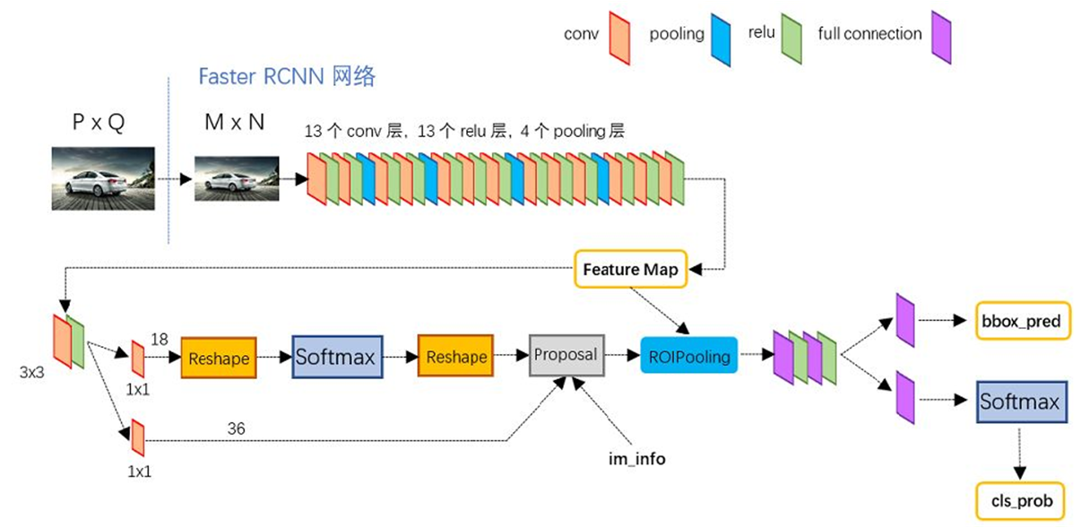
Think about adding more content here , See the picture below , It is Faster R-CNN A more detailed flow chart , Later, I will also tell you according to this structure , It should be clearer .
Feature extraction network
The structure of feature extraction network is shown in the figure below :
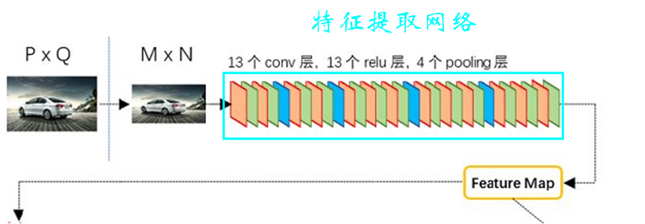
You can see , For one P*Q Size picture , Let's start with resize To specific M*N size , Then it is sent to the feature extraction network .【 notes : Here, the image size does not add the number of channels , Just understand 】
Besides , It can be seen that the feature extraction network in the figure has 13 Convolution layers ,4 A pool layer , In fact, this feature extraction network is famous VGG.【 notes : stay VGG There is 13 Convolution layers ,5 A pool layer , The last pooling layer is discarded here 】
about VGG Those unfamiliar with the network can click *** Learn more . It is worth mentioning that VGG In the network , Convolution uses 3*3 Convolution kernel , After convolution, the size of the characteristic image remains unchanged ; Pooling uses 2*2 The pooled core of , Halve the size of the characteristic map after pooling . in other words , In the feature extraction network in the figure above , It contains four pooling layers , Therefore, the size of the feature map we finally get is the original 1 16 \frac{1}{ {16}} 161, That is to say M 16 ∗ N 16 \frac{M}{ {16}}*\frac{N}{ {16}} 16M∗16N .
There's another point worth noting , That is, the feature extraction network in this explanation is VGG, We generally call it backbone( Backbone network ). This backbone It can be replaced as needed , Like changing into ResNet、MobileNet It's OK to wait .
RPN Network structure
RPN The network structure of is as follows :
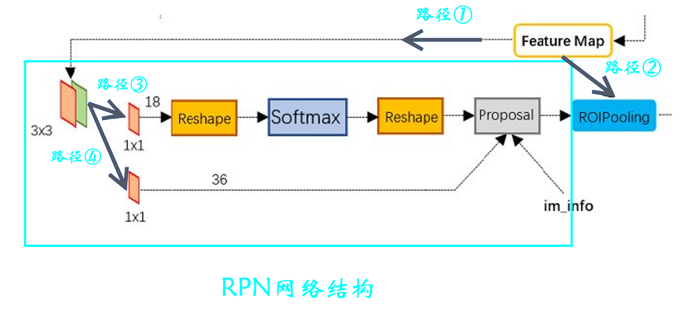
We have got the last step M 16 ∗ N 16 \frac{M}{ {16}}*\frac{N}{ {16}} 16M∗16N A feature map of size (Feature Map)【 notes : For the convenience of the following description , Now order W = M 16 , H = N 16 W=\frac{M}{ {16}},H=\frac{N}{ {16}} W=16M,H=16N】, We can see that we will make paths to the feature map respectively ① And the path ② The operating , The path ① The operation on is RPN Network structure . Now let's focus on this RPN Network structure .
First of all, let's clarify RPN What is it for ?enmmm…, If I don't know the function of this network now, I've really said it in vain , It's a bit of a failure . But this point cannot be overemphasized ——RPN Is to extract candidate boxes !!!
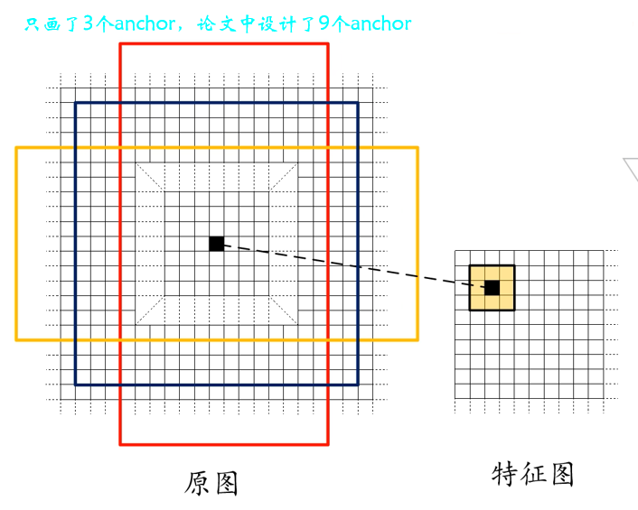
that RPN How do you do it ? First , We'll use a 3*3 The sliding window traverses the feature map just obtained , Then calculate the center point of the sliding window corresponding to the center point on the original image , Last in original image Draw each center point 9 Kind of anchor boxes .【 notes : How to get the center point of the original drawing from the center point coordinates of the feature drawing ?—— We're going to use VGG Backbone network , The size difference between the original drawing and the feature drawing 16 times , Therefore, you only need to multiply the coordinates of the center point of the feature map 16 that will do ; Or we can calculate the relative position of the center point in the feature map , Further get the central point of the original figure 】
We need to draw in the original picture 9 in anchor, Three scales are given in the paper (128*128 、256*256 、512*512) And three proportions (1:1、1:2、2:1) altogether 9 Kind of anchor, It is designed by experience , In fact, we can adjust according to the task in the implementation process , For example, the target we want to detect is small , Then it can be appropriately reduced anchor The size of the . The approximate mapping relationship between the center point of the feature map and the original map is as follows :
The use of 3*3 The sliding window traverses the characteristic graph , In fact, this corresponds to figure 4.1 route ① The first of 3*3 Convolution of , Convolution process padding=1,stride=1. Where the convolution and the original graph are generated anchor The corresponding relationship is shown in the figure below : It can be seen that after this step, we will generate many, many anchor, Obviously these anchor Many of them are not what we need , Later, we will talk about these anchor Make a choice .

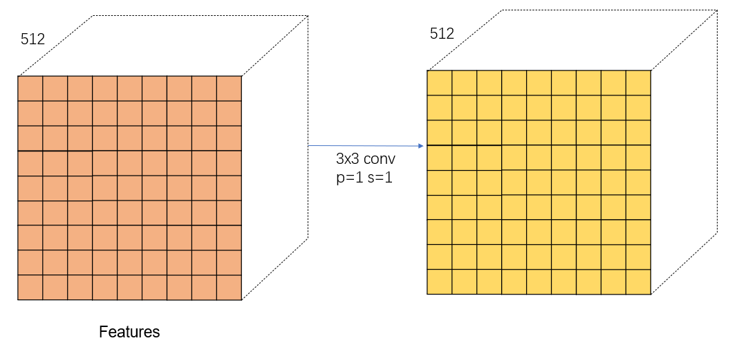
Next, let's see what happened 3*3 The change of characteristic graph after convolution , Because the convolution kernel is used k=3*3,p=1,s=1 Convolution of , Therefore, the size of the characteristic image does not change after convolution , Let's talk about this here channel=512 Is due to VGG The number of output channels of the last layer of the network is 512.
Then compare with the figure 4.1 have a look 3*3 After convolution of ?3*3 After convolution, the paths are taken separately ③ And the path ④ Carry out relevant operations . Actually path ③ Just got it anchor To classify ( Foreground and background ), And the path ④ That's right. anchor Fine tune the regression .
Then let's talk about it separately ③ and ④, First, let's talk about the path ③. Start with a 1*1 Convolution of , The number of convolution kernels is 18. As shown in the figure below :
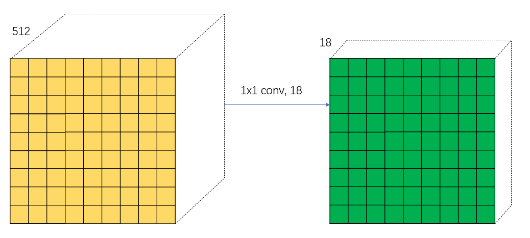
In fact, the above figure adopts 18 Convolution kernel is very particular . The first thing we need to know is the path ③ What we need to do is to distinguish each anchor Is it the foreground or the background , It is divided into two categories , For each small square, it will be generated on the original graph 9 individual anchor. such 2*9=18, Each small square in the result represents a certain position in the original image anchor Whether it is the probability of foreground or background . For your convenience , Pick out a square pair 18 Interpret the data of the channel , As shown in the figure below :
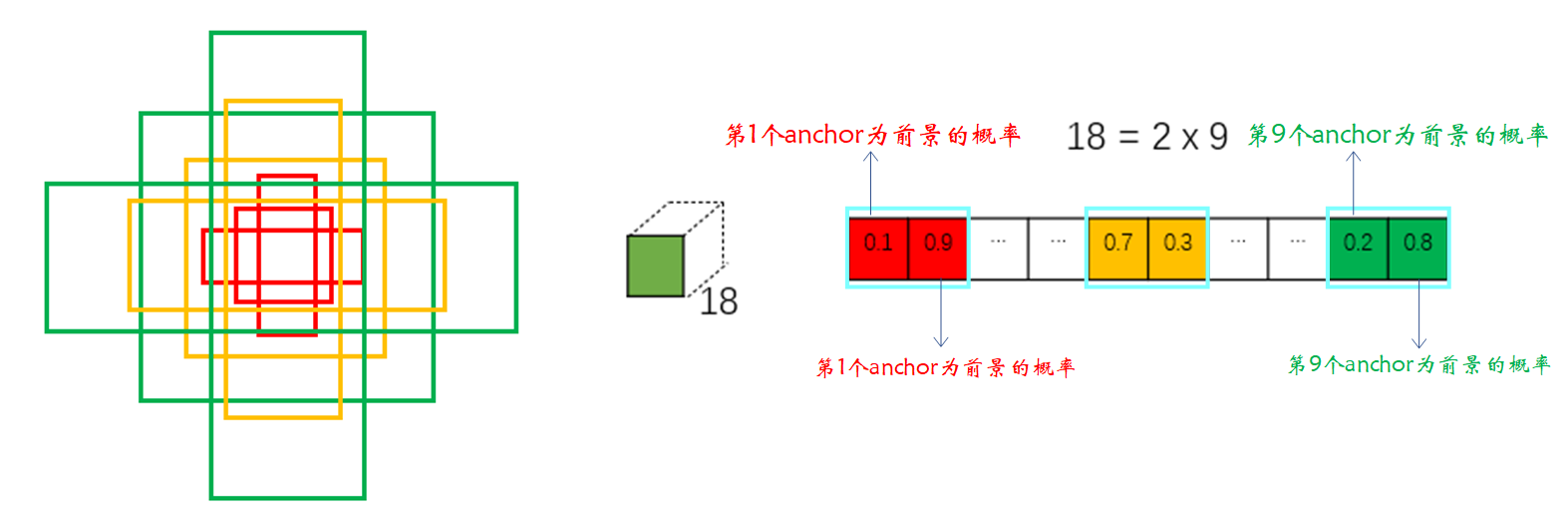
1*1 After convolution of , So it went on softmax Layer classification .【 notes : stay softmax There is one before and after the floor reshape The operation of , This is because there are requirements for the input format when writing code , Here you can not care about , The code will be described later 】 softmax After layer classification, we will get all positive classes anchor(positive anchors) And negative anchor(negative anchors).
Here we add the rules for selecting positive and negative samples : Positive samples have two conditions , First of all : Pick and true box IOU maximal anchor; second : Pick and true box IOU Greater than 0.7 Of anchor.【 notes : In fact, the second condition can be met in most cases , But condition one is set to prevent some extreme situations 】 The selection condition of negative samples is with all real boxes IOU All less than 0.3 Of anchor.
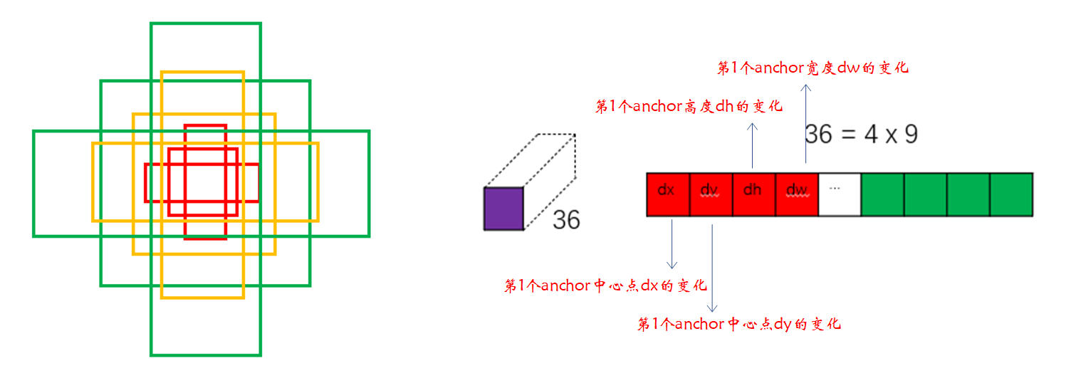
Then let's talk about the path ④, alike , First, there's a 1*1 Convolution of , The number of convolution kernels is 36. As shown in the figure below :
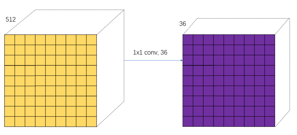
there 36 It's also exquisite , Because the regression is fine tuned anchor Every time anchor You need four parameters ,4*9=36, Each small square in the result represents a certain position in the original image anchor Four parameters that need to be adjusted . Also draw a picture to help you understand , as follows :
Next path ③ And the path ④ stay Proposal This step combines , What is this step for ? In fact! , This step is to integrate the path ③ And the path ④ Information in , That is, classification results and anchor Regression parameters of the box , The purpose is to get a more accurate candidate box (Region Proposal). Careful students may also find proposal There is another input in this step , namely im_info, This parameter saves some information about image size transformation , Like the beginning resize, Pool in the back and so on .
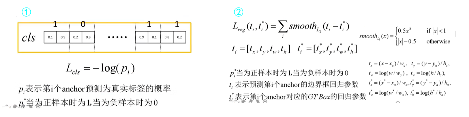
RPN Layer loss function
RPN The loss function of the layer is as follows :RPN Layer classification loss and fast R-CNN similar , It also consists of two parts , That is, classification loss and bounding box regression loss .
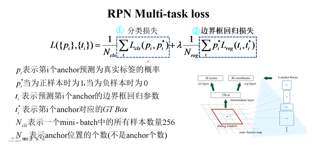
Let's take a specific look at ① and ② part :【 notes : Bounding box regression loss in the previous article R-CNN In the introduction , If you don't understand, you can find out 】
ROI Pooling
The above has been described in more detail RPN layer , That is, our figure 4.1 Medium ① route , Next, let's move on to the path ②【 route ② by ROI Pooling layer 】. You can see ROI Pooling There are two inputs to the layer : Respectively
- The original feature maps
- RPN Output proposal
ROI Pooling Layer I am fast R-CNN I've already talked about it in , There is not much to say here , Those who don't understand can go to recharge .
But here I still want to make a point : We passed ROI Pooling The input of the layer is the original feature map and RPN Output candidate box , We are equivalent to mapping each candidate box to different parts of the original feature map , Then cut these parts and pass them in ROI Poolinng layer .
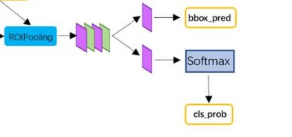
Classification regression fine tuning part
The latter part is actually completely related to Fast R-CNN The second half is exactly the same , Because we all passed by ROI Pooling Layer gets the relevant features of the candidate box , Then send it to the classification and regression network . If you don't understand this part, please read my previous article on this part .
Summary
In this part, let's summarize Faster R-CNN Steps for , as follows :
- Input the complete image into the network to get the corresponding feature map
- Use RPN Structure generation candidate box , take RPN The generated candidate frame is projected onto the original feature map to obtain the corresponding feature matrix 【 It's equivalent to us ROI Pooling Some of the results obtained by clipping 】
- The characteristic matrix is ROI pooling Layers are scaled to uniform size , Then flatten the characteristic map to get the prediction result
thus ,Faster R-CNN The theoretical part of will be over , I hope everyone can get something .
Reference material
Faster RCNN A collection of theories
If the article is helpful to you , It would be
Whew, whew, whew ~~duang~~ A great bai
边栏推荐
- Database SQL practice 4. Find the last of employees in all assigned departments_ Name and first_ name
- Mipi interface, DVP interface and CSI interface of camera
- Ros2 - install ros2 (III)
- *P++, (*p) + +, * (p++) differences
- [solved] there is something wrong with the image
- M2dgr slam data set of multi-source and multi scene ground robot
- ethtool 原理介绍和解决网卡丢包排查思路(附ethtool源码下载)
- [vscode] prohibit the pylance plug-in from automatically adding import
- SOC_ SD_ CMD_ FSM
- Binary search (half search)
猜你喜欢
. Net core stepping on the pit practice
Ethtool principle introduction and troubleshooting ideas for network card packet loss (with ethtool source code download)
ethtool 原理介绍和解决网卡丢包排查思路(附ethtool源码下载)
PHY驱动调试之 --- PHY控制器驱动(二)

数学分析_笔记_第8章:重积分
一文揭开,测试外包公司的真实情况
window navicat连接阿里云服务器mysql步骤及常见问题
Logical structure and physical structure
An article was opened to test the real situation of outsourcing companies
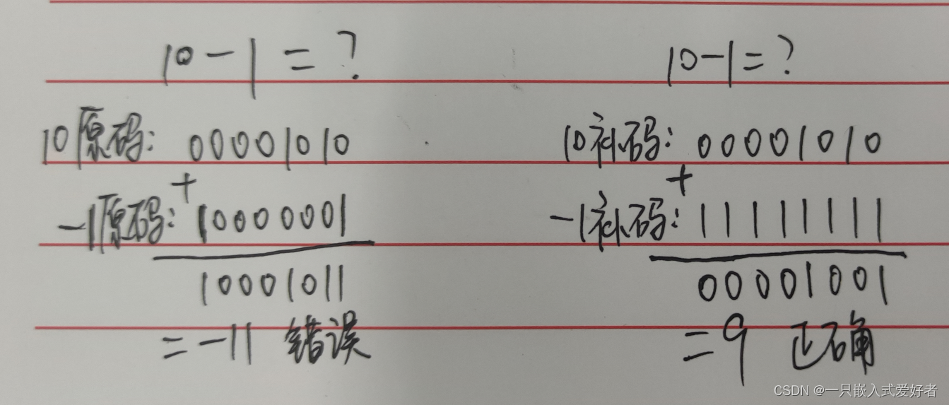
Negative number storage and type conversion in programs
随机推荐
Orin two brushing methods
小米笔试真题一
三体目标管理笔记
U-Boot初始化及工作流程分析
2022年中纪实 -- 一个普通人的经历
D2L installation
解读最早的草图-图像翻译工作SketchyGAN
[OBS] x264 Code: "buffer_size“
一文揭开,测试外包公司的真实情况
[MySQL 8.0 does not support capitalization of table names - corresponding scheme]
[software testing] 06 -- basic process of software testing
C learning notes
Xavier CPU & GPU high load power consumption test
ROS2——安装ROS2(三)
SD_CMD_SEND_SHIFT_REGISTER
【软件测试】06 -- 软件测试的基本流程
Unity UGUI不同的UI面板或者UI之间如何进行坐标匹配和变换
Netease to B, soft outside, hard in
数学分析_笔记_第8章:重积分
[vscode] prohibit the pylance plug-in from automatically adding import