Safety reinforcement learning based on linear function approximation safe RL with linear function approximation translation 2

The paper ：Safe Reinforcement Learning with Linear Function Approximation
Download address ：http://proceedings.mlr.press/v139/amani21a/amani21a.pdf
meeting / year ：PMLR / 2021

Word Version download address （ Hard work ）：https://download.csdn.net/download/baishuiniyaonulia/85863332
The translation of this article belongs to semi manual , Please forgive me for any mistakes .

Abstract 、1、2、3

Safety reinforcement learning based on linear function approximation Safe RL with Linear Function Approximation translate 1 —— https://blog.csdn.net/baishuiniyaonulia/article/details/125504660

4. Extend to randomized policy choices Extension to randomized policy selection

The first 2 Section SLUCB-QVI Only deterministic strategies can be output . In this section , We show that our results can be extended to the setting of random policy selection , This may be desirable in practice . Random strategy $\pi :\mathcal{S}\times [H]\to {\Delta }_{\mathcal{A}}$ Map States and time steps to distributions on actions , bring $a\sim \pi (s,h)$ It's a strategy π It is suggested that the agent is in a state $s\in \mathcal{S}$ Time is in the time step $h\in [H]$ The action performed . In every plot k And time steps $h\in [H]$ in , When in state $s_h^k$ when , The agent must start from a Extract its action $a_h^k$ The security policy ${\pi }_k\left(s_h^k,h\right)$ bring $${\mathbb{E}}_{a_h^k\sim {\pi }_k\left(s_h^k,h\right)}{c}_h\left(s_h^k,a_h^k\right)\le \tau$$ The probability is high . Accordingly, we define a set of unknown security policies $${\tilde{\Pi }}^{\text{safe }}:=\left\{\pi :\pi (s,h)\in {\Gamma }_h^{\text{safe }}(s),\forall (s,h)\in \mathcal{S}\times [H]\right\}$$

among ${\Gamma }_h^{\text{safe}}(s):=\left\{\theta \in {\Delta }_{\mathcal{A}}:{\mathbb{E}}_{a\sim \theta }{c}_h(s,a)\le \tau \right\}$. therefore , In the k Time step of round $h\in [H]$ Observation state $s_h^k$ after , The strategy selection of the agent must belong to ${\Gamma }_h^{\text{safe}}(s_h^k)$ The probability is high . In this formula , Strategy π Of （ action ） The expected value in the definition of value function exceeds the environment and strategy π The randomness of . We use it ${\tilde{V}}_h^{\pi }$ and ${\tilde{Q}}_h^{\pi }$ To represent them , Distinguish from ${\tilde{V}}_h^{\pi }$ and ${\tilde{Q}}_h^{\pi }$ stay (2) and (3) In the definition of , For deterministic strategies π. Make ${\pi }_{\ast }$ Is the optimal security policy , bring ${\tilde{V}}_h^{{\pi }_{\ast }}(s):={\tilde{V}}_h^{\ast }(s)=\underset{\pi \in {\tilde{\Pi }}^{\text{safe }}}{\sup }{\tilde{V}}_h^{\pi }(s)$ For all $(s,h)\in \mathcal{S}\times [H]$. therefore , For all $(a,s,h)\in \mathcal{A}\times \mathcal{S}\times [H]$, Behrman equation of security policy $\pi \in {\tilde{\Pi }}^{\text{safe }}$ And the optimal security policy is

$$\begin{array}{rl}& {\tilde{Q}}_h^{\pi }(s,a)=r_h(s,a)+\left[{\mathbb{P}}_h{\tilde{V}}_{h+1}^{\pi }\right](s,a),\\ & {\tilde{V}}_h^{\pi }(s)={\mathbb{E}}_{a\sim \pi (s,h)}\left[{\tilde{Q}}_h^{\pi }(s,a)\right],\end{array}$$$$\begin{array}{rl}& {\tilde{Q}}_h^{\ast }(s,a)=r_h(s,a)+\left[{\mathbb{P}}_h{\tilde{V}}_{h+1}^{\ast }\right](s,a),\\ & {\tilde{V}}_h^{\ast }(s)={\max }_{\theta \in {\Gamma }_h^{\text{safe }(s)}}{\mathbb{E}}_{a\in \theta }\left[{\tilde{Q}}_h^{\ast }(s,a)\right],\end{array}$$

among ${\tilde{V}}_{H+1}^{\pi }(s)={\tilde{V}}_{H+1}^{\ast }(s)=0$, Defines cumulative regret Such as $R_K:=\sum _{k=1}^K{\tilde{V}}_1^{\ast }(s_1^k)-{\tilde{V}}_1^{{\pi }_k}(s_1^k)$. (11) The definition of security constraints in enables us to get rid of the set $\mathcal{D}(s):=\{\varphi (s,a):a\in \mathcal{A}\}$ Star convexity hypothesis （ hypothesis 5）, This is necessary for the deterministic strategy selection method . We suggest that SLUCB-QVI Make changes , To adapt to this new formula , It's called random SLUCB-QVI (RSLUCB-QVI). This new algorithm also realizes the comparison with SLUCB-QVI Sublinear regret of the same order , namely $\tilde{\mathcal{O}}\left(\kappa \sqrt{d^3{H}^{3}T}\right)$.

Although with SLUCB-QVI（ See （1）） Compared with the safety constraints considered in ,RSLUCB-QVI Respect the more moderate definition of security constraints （ See （11））, But it is still better than other existing algorithms through random strategy selection CMDP Has significant advantages （Efroni wait forsomeone ,2020;Turchetta wait forsomeone ,2020;Garcelon wait forsomeone ,2020;Zheng and Ratliff,2020;Ding wait forsomeone ,2020a;Qiu wait forsomeone ,2020;Ding wait forsomeone ,2020b;Xu wait forsomeone ,2020 year ;Kalagarla wait forsomeone ,2020 year ）. First , The security constraints considered in these algorithms are defined by the cumulative expected cost in the time range below a certain threshold , and RSLUCB-QVI Make sure that at every time step of the action （ Not in a time frame ） Expected costs incurred Less than threshold . secondly , Even this looser definition of safety constraints , The best method that these algorithms can guarantee in terms of constraint satisfaction is the sublinear limit of the number of constraint violations , and RSLUCB-QVI Make sure there is no constraint violation .

4.1. Random SLUCB-QVI Randomized SLUCB-QVI

We now describe the algorithm 2 As summarized in RSLUCB-QVI. Make ${\varphi }^{\theta }(s):={\mathbb{E}}_{a\sim \theta }\varphi (s,a)$. In every plot $k\in [K]$ in , In the first cycle , Agents calculate all $s The real unknown set of ${\Gamma }_h^{\text{safe}}(s)$ Estimation set of $s\in \mathcal{S}$ as follows ：
$${\Gamma }_h^k(s):=\{\theta \in {\Delta }_{\mathcal{A}}:{\mathbb{E}}_{a\sim \theta }\left[\frac{*{\Phi }_0(s,\varphi (s,a)),\tilde{\varphi }\left(s,a_0(s)\right)*}{{\Vert \varphi \left(s,a_0(s)\right)\Vert }_2}{\tau }_h(s)\right]+\underset{\nu \in {\mathcal{C}}_h^k(s)}{\max }*{\Phi }_0^{\perp }\left(s,{\mathbb{E}}_{a\sim \theta }[\varphi (s,a)]\right),\nu *\le \tau \}$$

$$=\left\{\theta \in {\Delta }_{\mathcal{A}}:\frac{*{\Phi }_0\left(s,{\varphi }^{\theta }(s)\right),\tilde{\varphi }\left(s,a_0(s)\right)*}{{\Vert \varphi \left(s,a_0(s)\right)\Vert }_2}{\tau }_h(s)+*{\gamma }_{h,s}^k,{\Phi }_0^{\perp }\left(s,{\varphi }^{\theta }(s)\right)*+\beta {\Vert {\Phi }_0^{\perp }\left(s,{\varphi }^{\theta }(s)\right)\Vert }_{{\left({\mathbf{A}}_{h,s}^k\right)}^{-1}}\le \tau \right\}$$

Please note that , because MDP The linear structure of , We can go through the linear form again $*{\tilde{\mathbf{w}}}_h^{\ast },\varphi (s,a)*$ A parameterized ${\tilde{Q}}_h^{\ast }(s,a)$ , among ${\tilde{\mathbf{w}}}_h^{\ast }:={\theta }_h^{\ast }+{\int }_{\mathcal{S}}{\tilde{V}}_{h+1}^{\ast }(s^{\prime })d\mu (s^{\prime })$. In the next step , For all $(s,a)\in \mathcal{S}\times \mathcal{A}$, Agent computing $${\tilde{Q}}_h^k(s,a)=*{\tilde{\mathbf{w}}}_h^k,\varphi (s,a)*+{\kappa }_h(s)\beta {\Vert \varphi (s,a)\Vert }_{{\left({\mathbf{A}}_h^k\right)}^{-1}}$$

among ${\tilde{\mathbf{w}}}_h^{\ast }:={\left({\mathbf{A}}_h^k\right)}^{-1}widetilde{\mathbf{b}}_h^k$ By Gram matrix $ Calculated ${\tilde{\mathbf{w}}}_h^{\ast }$ Regularized least squares estimator of \mathbf{A}_{h}^{k}$ and ${\tilde{\mathbf{b}}}_h^k:=\sum _{j=1}^{k-1}{\varphi }_h^j\left[r_h^j+\min \left\{{\max }_{\theta \in {\Gamma }_{h+1}^k\left(s_{h+1}^j\right)}{\mathbb{E}}_{a\sim \theta }\left[{\tilde{Q}}_{h+1}^k\left(s_{h+1}^j,a\right)\right],H\right\}\right]$. After these calculations in the first cycle , Agents are distributed ${\Gamma }_h^k\left(s_h^k\right)$ Draw actions in $a_h^k$ In the second cycle . Definition ${\tilde{V}}_h^k(s):=\min \left\{{\max }_{\theta \in {\Gamma }_h^k(s)}{\mathbb{E}}_{a\sim \theta }\left[{\tilde{Q}}_h^k(s,a)\right],H\right\}$ , and ${\mathcal{E}}_3:=\{|*{\tilde{\mathbf{w}}}_h^k,\varphi (s,a)*-{\tilde{Q}}_h^{\pi }(s,a)-\left[{\mathbb{P}}_h{\tilde{V}}_{h+1}^{\pi }-{\tilde{V}}_{h+1}^k\right](s,a)|\le \beta {\Vert \varphi (s,a)\Vert }_{{\left({\mathbf{A}}_h^k\right)}^{-1}},\forall (a,s,h,k)\in \mathcal{A}\times \mathcal{S}\times [H]\times [K]\}$.

It can be easily proved , Theorem 2 The results described in apply to settings that focus on random strategies , That is to say 1、2、3 and 4 Next , And according to the theorem 1 in β The definition of , The probability is at least $1-2\delta$, event $\tilde{\mathcal{E}}:={\mathcal{E}}_1\bigcap {\mathcal{E}}_3$ establish . therefore , As a proposition 1 The direct conclusion of , Promise to ${\mathcal{E}}_1$ On condition that ,${\Gamma }_h^k(s)$ All policies within are secure , namely ${\Gamma }_h^k(s)\subset {\Gamma }_h^{\text{safe}}(s)$. Now? , In the following lemma , We quantified ${\kappa }_h(s)$.

lemma 2 （ face RSLUCB-QVI Optimistic attitude towards safety constraints ） Lemma 2 (Optimism in the face of safety constraint in RSLUCB-QVI)

Make ${\kappa }_h(s):=\frac{2H}{\tau -{\tau }_h(s)}+1$ And assumptions 1,2,3 ,4 keep . then , With events $\tilde{\mathcal{E}}$ On condition that , It thinks ${\tilde{V}}_h^{\ast }(s)\le {\tilde{V}}_h^k(s),\forall (s,h,k)\in \mathcal{S}\times [H]\times [K]$.

The certificate is contained in Appendix B.1 in . Using lemmas 2, We prove ${\tilde{Q}}_h^{\ast }(s,a)\le {\tilde{Q}}_h^k(s,a)$, $forall(a,s,h,k)\in \mathcal{A}\times \mathcal{S}\times [H]\times [K]$. This highlights the RSLUCB-QVI Of UCB characteristic , So that we can take advantage of unsafe LSVI-UCB (Jin et al., 2020) Standard analysis to establish regret circles .

Theorem 3 （RSLUCB-QVI Regret of ） Theorem 3 (Regret of RSLUCB-QVI)

Assuming 1、2、3 and 4 Next , There is an absolute constant $c_{\beta }>0$ So that for any fixed $\delta \in (0,1/3)$, also Theorem 1 in β The definition of , If we set ${\kappa }_h(s):=\frac{2H}{\tau -{\tau }_h(s)}+1$,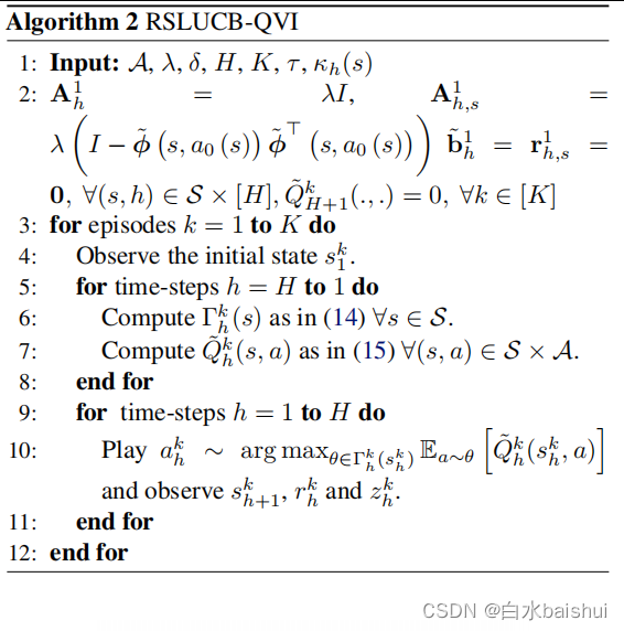

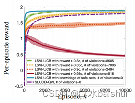
chart 1. SLUCB-QVI Comparison and verification with unsafe state-of-the-art technology ：1) When LSVI-UCB (Jin et al., 2020) know ${\gamma }_h^{\ast }$ , It is expected to be better than SLUCB-QVI（ I do not know! ${\gamma }_h^{\ast }$）; 2） When LSVI-UCB I do not know! ${\gamma }_h^{\ast }$（ Such as SLUCB-QVI The situation of ） And its goal is to maximize $r-{\lambda }^{\prime }c$ instead of r , The larger ${\lambda }^{\prime }$ As a result, the number of reward and constraint violations per round is small , and SLUCB-QVI The number of constraint violations for is zero .

Then at least $1-3\delta$ Probability , It thinks $R_K\le 2H\sqrt{T\log \left(\frac{dT}{\delta }\right)}+2(1+\kappa )\beta \sqrt{2dHT\log \left(1+\frac{K}{d\lambda }\right)}$, among $\kappa :={\max }_{(s,h)\in \mathcal{S}\times [H]}{\kappa }_h(s)$. The certificate is attached in Appendix B.2.

5. experiment Experiments

In this section , We propose numerical simulation to supplement and confirm our theoretical findings . We evaluate SLUCB-QVI Performance in synthetic environments , And in OpenAI Gym Of Frozen Lake Implement... In the environment RSLUCB-QVI（Brockman wait forsomeone ,2016 year ）.

5.1. In synthetic environment SLUCB-QVI SLUCB-QVI on synthetic environments

chart 1 The results shown in describe 20 Average value of times realized , So we chose $\delta =0.01,\sigma =0.01,\lambda =1,d=5,\tau =0.5,H=3$ and $K= 10000 dollar . Parameters ${\left\{{\theta }_h^{\ast }\right\}}_{h\in [H]}$ and ${\left\{{\gamma }_h^{\ast }\right\}}_{h\in [H]}$ come from $\mathcal{N}\left(0,I_d\right)$. To tune parameters ${\left\{{\mu }_h^{\ast }(.)\right\}}_{h\in [H]}$ And feature maps $\varphi$ such They are related to assumptions 1 compatible , We think that feature space $\{\varphi (s,a):(s,a)\in \mathcal{S}\times \mathcal{A}\}$ Is a subset d Dimensional simplex and ${\mathbf{e}}_i^{\top }{\mu }_h^{\ast }(.)$ It's right $\mathcal{S}$ Any probability measure of all $i\in [d]$. This guarantees the assumption 1 establish .

stay SLUCB-QVI The first cycle of （ The first 6 That's ok ） Calculate the security set in ${\mathcal{A}}_h^k(s)$, Then choose the action of maximizing the linear function （ In feature mapping $ \phi $) In feature space ${\mathcal{D}}_h^k\left(s_h^k\right):=\left\{\varphi \left(s_h^k,a\right):a\in {\mathcal{A}}_h^k\left(s_h^k\right)\right\}$ In the second cycle （ The first 10 That's ok ）. Unfortunately , Even if the feature space $\{\varphi (s,a):(s,a)\in \mathcal{S}\times \mathcal{A}\}$ It's convex , aggregate ${\mathcal{D}}_h^k\left(s_h^k\right)$ Can have forms that are difficult to maximize linear functions . In our experiment , We define mapping $\phi $ Make the set $\mathcal{D}(s)$ stay $\varphi \left(s,a_0(s)\right)$ And $N=100$ （ See definition 1）, therefore , We can prove that SLUCB-QVI Of the 10 The optimization problem in the row can be effectively solved （ See appendix C The proof of ）.

Definition 1 （ Finite star convex set ） Definition 1 (Finite star convex set)

Around one $x_0\in {\mathbb{R}}^d$ Star convex set of $\mathcal{D}$ It is limited. , If there are finite vectors ${\left\{{\mathbf{x}}_i\right\}}_{i=1}^N$ bring $\mathcal{D}={\bigcup }_{i=1}^N\left[{\mathbf{x}}_0,{\mathbf{x}}_i\right]$, among $\left[{\mathbf{x}}_0,{\mathbf{x}}_i\right]$ Is the connection ${\mathbf{x}}_0$ and ${\mathbf{x}OfLine}_i$.

chart 1 It depicts SLUCB-QVI The average reward per round , And compare it with the baseline , And emphasized SLUCB-QVI Value in respecting the safety constraints of all time steps . say concretely , We will SLUCB-QVI And 1) LSVI-UCB (Jin et al., 2020) Compare , Because it has knowledge of security constraints , namely ${\gamma }_h^{\ast }$; 2) LSVI-UCB, When it doesn't know ${\gamma }_h^{\ast }$（ Such as SLUCB-QVI The situation of ） And its goal is to maximize the function $r-{\lambda }^{\prime }c$, Constraints are pushed into the objective function , about ${\lambda }^{\prime }=0.8,0.85,0.9$ and 0.95 Different values of . therefore , Discourage costly actions through low incentives . The figure verifies that ${\gamma }_h^{\ast }$ Knowledgeable LSVI-UCB I don't know ${\gamma }_h^{\ast }$ Better than... As expected SLUCB-QVI. Besides , When LSVI-UCB Trying to maximize $r-{\lambda }^{\prime }c$（ I do not know! ${\gamma }_h^{\ast }$) and SLUCB-QVI The number of constraint violations of is zero .

5.2. Frozen lake environment RSLUCB-QVI RSLUCB-QVI on Frozen Lake environment

We assessed RSLUCB-QVI stay Frozen Lake Performance in the environment . Agents seek to 10 × 10 2D Achieve the goal in the map （ chart 2a）, At the same time, avoid danger .

chart 2.RSLUCB-QVI and CISR (Turchetta et al., 2020) stay Frozen Lake Comparison in the environment .

At each time step , Agents can move in four directions , namely $\mathcal{A}=\{a_1:\text{left, }{a}_2:\text{right, }{a}_3:\text{down, }{a}_4:\text{up}\}$. It uses 0.9 The probability of moving in the desired direction , With 0.05 The probability of moving in any orthogonal direction . We set up $H=1000,K=10,d=|\mathcal{S}|=100$, AND${\mu }^{\ast }(s)\sim \mathcal{N}\left(0,I_d\right)$ for all $s\in \mathcal{S}=\left\{s_1,\dots ,s_{100}\right\}$. then , We correctly specify all by solving a set of linear equations $(s,a)\in \mathcal{S}\times \mathcal{A}$ Feature mapping of $\varphi (s,a)$, Make the transformation respect the details of the above environment . In order to interpret the requirement of avoiding danger as a form (11) Constraints , We will ${\gamma }^{\ast }$ and $\tau $ The adjustment is as follows ： The cost of performing actions $a\in \ state $s\in \mathcal{S}$ Situated mathcal{A}$ Is the probability that the agent moves to one of the dangerous states . therefore , The security policy ensures that the expected value of the probability of moving to a dangerous state is a small value . So , We set up ${\gamma }^{\ast }=\sum _{s\in \text{ Danger states }}{\mu }^{\ast }(s)$ and $\tau =0.1$. Besides , For each state $s\in \mathcal{S}$, Will be a safe action , That is, it leads to a small probability （$\tau =0.1$） One of the dangerous states of the game is given to the agent . We solve a set of linear equations to adjust ${\theta }^{\ast }$, Make in every state $s\in \mathcal{S}$, The direction to the state closest to the goal state to agent Reward 1, And play the other three directions to reward it 0.01. The model persuades agents to move towards their goals .

In the specified characteristic diagram $\varphi$ And adjust all parameters , We are 10 Interaction units （episodes）（ namely $K=10$） Realized RSLUCB-QVI, Each interaction unit consists of 1000 Time steps （horizon） form , namely $H= 1000 dollar ）. In each interaction unit （ The plot ） During and after each move , The agent can finally be in one of the following three states ：1） The goal is , This leads to the successful termination of the interaction unit ; 2) dangerous , Cause the interaction unit to fail and then terminate ; 3） Security . The agent will receive 6 The return of , Or you'll get 0.01.

In the figure 2 in , We reported more than 20 The average success rate and return of agents , We implemented for each agent 10 Time RSLUCB-QVI, And compare our results with (Turchetta et al., 2020) Proposed CISR The results are compared , Among them, the teacher provided help Agents choose safe actions through intervention . although RSLUCB-QVI and CISR The performance of these two methods is equivalent , But the important thing to consider is ,CISR Each interaction unit in （ The plot ） from 10000 Time steps , And in the RSLUCB-QVI The number in is 1000 individual . It is worth noting that ,RSLUCB-QVI Learning rate ratio CISR fast . It is also worth noting that , When using optimization intervention, we will RSLUCB-QVI And CISR Made a comparison , Compared with other types of interventions , It gives the best result .

6. Conclusion Conclusion

In this paper , We developed SLUCB-QVI and RSLUCB-QVI, These two kinds of safety RL The algorithm is linear at finite level MDP In the setting of . For these algorithms , We provide a sublinear regret boundary $\tilde{\mathcal{O}}\left(\kappa \sqrt{d^3{H}^{3}T}\right)$, among H Is the duration of each episode ,d Is the dimension of feature mapping ,κ Is a constant that characterizes security constraints ,$T=KH$ Is the total number of action scenes . We have proved that they will probably never violate unknown security constraints . Last , We are synthesizing and Frozen Lake In the environment SLUCB-QVI and RSLUCB-QVI, This proves that our algorithm has the same performance as the algorithms that understand security constraints or use existing technology Teacher advice to help agents avoid unsafe behavior .