Chapter 7 Bayesian classifier

1. Explain a priori probability 、 Posterior probability 、 All probability formula 、 Conditional probability formula , The Bayesian formula is illustrated with examples , How to understand Bayesian theorem ？

• Prior probability
  Prior probability $P(c)$ It expresses the proportion of various samples in the sample space , According to the law of large numbers , When the training set contains sufficient independently distributed samples ,$P(c)$ It can be estimated by the frequency of occurrence of various samples .
• Posterior probability
  Delay probability $P(c|x)$, It can be understood as in category $c$ In the training set $x$ The so-called “ The probability of real occurrence ”
• All probability formula
  
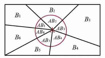
  As shown in the figure , A sample space $S$ By $B_1,B_2...B_6$ Such a complete event group is perfectly divided , Events marked in the red circle $A$ It has also been ruthlessly decomposed into various parts , Now our fragmented event $A$ Put it together ：
  $$\begin{gathered} P(A)=P(A{B}_1)+P(A{B}_2)+...+P(A{B}_6) \\ =P(A|B_1)P(B_1)+P(A|B_2)P(B_2)+...P(A|B_6)P(B_6) \end{gathered}$$
• Conditional probability formula
  $P(A|B)$ In the event of $B$ Under the condition of occurrence , event $A$ Probability of occurrence
• Bayes' formula
  $$P(B_i|A)=\frac{P(B_{i}A)}{P(A)}=\frac{P(A|B_i)P(B_i)}{{\sum }_{j=1}^{n}P(A|B_j)P(B_j)}$$
  In a nutshell , Bayesian theorem is a priori probability based on hypothesis 、 The probability of observing different data under given assumptions , A method for calculating a posteriori probability is provided .

2. An example is given to illustrate how naive Bayesian classifier classifies test samples ？ And summarize the algorithm steps .

Naive Bayes is an independent expression of Bayesian evidence , It belongs to a special case . Bayesian expression is very complex in practical application , But we hope to split it into several naive Bayes to express , In this way, the posterior probability can be obtained quickly .

The basic idea of naive Bayes ： For a given item to be classified $x${ $x1,x2,...xn$} , Solve each category under the conditions appearing in this item $c_i$ Probability of occurrence . Which one? $P(c_i|x)$ Maximum , Which category does the item to be classified belong to .
Algorithm steps ：

• 1
  One for each data sample n Dimension eigenvector $x=$ { $x1,x2,...xn$} Express , Describe the right n Attributes $A1,A2,...An$ Of the sample n A measure .

• 2
  Suppose there is m Classes $c_1,c_2,...,c_m$ , Given an unknown data sample $x$, The classifier will predict $x$ It belongs to the class with the highest a posteriori probability . in other words , Naive Bayesian classification assigns unknown samples to classes $c_i(1⩽i⩽m)$ If and only if $P(c_i|x)>P(c_j|x)i\ne j$ . such , Maximize $P(c_i|x)$. Its $P(c_i|x)$ The largest class $c_i$ It is called the maximum a posteriori assumption . According to Bayes theorem ：
  $$P(c_i|x)=\frac{P(x|c_i)P(c_i)}{P(x)}$$

• 3
  because $P(x)$ Constant for all classes , It only needs $P(x|c_i)P(c_i)$ The biggest one is . If $c_i$ The prior probability of the class is unknown , It is usually assumed that these classes are equal probability , namely $P(c_1)=P(c_2)=...=P(c_m)$ , So it turns into right $P(x|c_i)$ To maximize （$P(x|c_i)$ It is often called given $c_i$ Time data $x$ The likelihood of , And make $P(x|c_i)$ The biggest assumption $c_i$ It is called maximum likelihood . otherwise , Need to maximize $P(x|c_i)P(c_i)$. Be careful , The prior probability of a class can be used $P(c_i)=s_i/s$ Calculation , among $s_i$ yes $c_i$ Number of training samples in , $s$ Is the total number of training samples .

• 4
  Given a dataset with many attributes , Calculation $P(x|c_i)$ The cost of can be very large . To reduce the calculation $P(x|c_i)$ The cost of , We can make the simple assumption of class conditional independence . The class label of the given sample , Assume that attribute values are conditionally independent of each other , That is, between attributes , There are no dependencies . In this way, only molecules need to be considered ：
  $$P(x|c_i)=\prod _{k=1}^{n}P(x_k|c_i)$$

• 5
  For unknown samples $x$ classification , That is, for each class $c_i$, Calculation $P(x|c_i)P(c_i)$ , Naive Bayesian classification assigns unknown samples to classes $c_i(1⩽i⩽m)$ If and only if $P(c_i|x)>P(c_j|x)i\ne j$ . such , $x$ Assigned to its $P(x|c_i)P(c_i)$ The largest class .
  The flow chart is shown in the figure below ：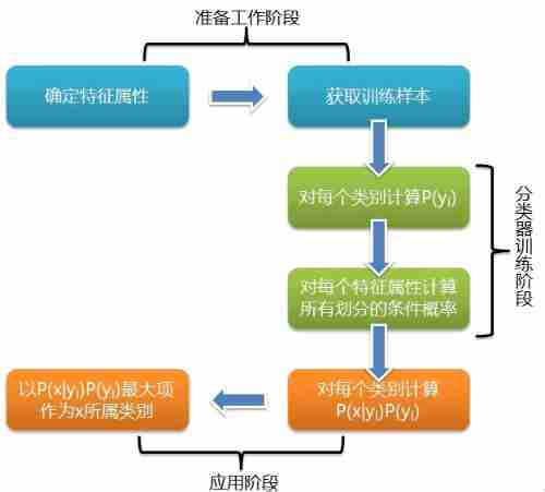
  

• The example analysis
  There is a batch of products of the same model , It is known that the production of one factory accounts for 15%, The production of the second factory accounts for 80%, The production of the three plants accounts for 5%, It is also known that the defective rates of these three factories are 2%,1%,3%. Any one of these products is defective , Ask which factory this defective product belongs to with the greatest probability ：
  set up $A$ Express “ What I got was a defective one ”,$B_i$ Express “ The defective products obtained are from i Provided by factory ”, be $B_1,B_2,B_3$ It's sample space $\Omega$ A division of , And $P(B_1)=0.5,P(B_2)=0.80,P(B_3=0.05)$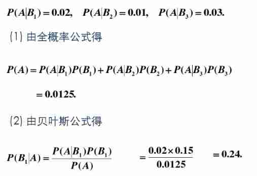
  
  
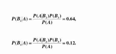
  thus it can be seen , The probability from factory two is the highest .

3. Explain how to use maximum likelihood estimation and Bayesian estimation to estimate the parameters of naive Bayes .

• Maximum likelihood estimation
  Maximum likelihood estimate the parameters to be estimated $\theta$ It is regarded as an unknown variable in a fixed form , Then we combine the real data to solve this fixed form of position variable by maximizing the likelihood function . The specific solving process is as follows ：

• Hypothesis sample set $D=$ { $x_1,x_2,...x_n$}, Suppose that the samples are relatively independent , So there is ：
  $$P(D|\theta )=P(x_1|\theta )P(x_2|\theta )...P(x_n|\theta )$$
  So suppose the likelihood function is ：
  $$L(\theta |D)=\prod _{k=1}^{n}P(x_k|\theta )$$
  Next, our criterion for finding parameters is to maximize the likelihood function as the name ：
  $$\theta =arg\underset{\theta }{\max }L(\theta |D)$$

• Bayesian estimation
  Bayesian estimation treats parameters as random variables with a known prior distribution , This means that this parameter is not a fixed unknown , It conforms to a certain prior distribution, such as ： A random variable $\theta$ Conform to normal distribution, etc .
  - Finally, Bayesian estimation is also to obtain a posteriori probability , What it ultimately derives is ：
  $$P(w_i|x,D)=\frac{P(w_i|x,D)}{P(x,D)}=\frac{P(w_i,x,D)}{{\sum }_{j=1}^{c}P(w_i,x,D)}$$
  There are in the above formula ：
  $$P(w_i,x,D)=\frac{P(x|w_i,D)P(w_i)}{{\sum }_{j=1}^{c}P(w_i,x,D)}$$
  There is also an important assumption , That is, the samples are independent of each other , At the same time, classes are also independent , So there are the following assumptions ：
  $$\begin{gathered} P(w_i|D)=P(w_i) \\ P(x|w_i,D)=P(x|w_i,D_i) \end{gathered}$$
  At the same time, because classes are independent of each other , Then there is ：
  $$P(x|w_i,D_i)=P(x|D)$$
  Similar to the derivation of maximum likelihood function , Available ：
  $$P(D|\theta )=\prod _{k=1}^{n}P(x_k|\theta )$$
  So we finally get ：
  $$P(x|D)=\int P(x|\theta )P(\theta |D)d\theta$$

4. Programming Laplace modified naive Bayesian classifier , And watermelon dataset 3.0 For example （P84）, Yes P151 Test samples of 1 To judge .

// An highlighted block
import xlrd
import math

class LaplacianNB():
    """
    Laplacian naive bayes for binary classification problem.
    """
    def __init__(self):
        """
        """

    def train(self, X, y):
        """
        Training laplacian naive bayes classifier with traning set (X, y).
        Input:
            X: list of instances. Each instance is represented by 
            y: list of labels. 0 represents bad, 1 represents good.
        """
        N = len(y)
        self.classes = self.count_list(y)
        self.class_num = len(self.classes)
        self.classes_p = {
    }
        #print self.classes
        for c, n in self.classes.items():
            self.classes_p[c] = float(n+1) / (N+self.class_num)

        self.discrete_attris_with_good_p = []
        self.discrete_attris_with_bad_p = []
        for i in range(6):
            attr_with_good = []
            attr_with_bad = []
            for j in range(N):
                if y[j] == 1:
                     attr_with_good.append(X[j][i])
                else:
                    attr_with_bad.append(X[j][i])
            unique_with_good = self.count_list(attr_with_good)
            unique_with_bad = self.count_list(attr_with_bad)
            self.discrete_attris_with_good_p.append(self.discrete_p(unique_with_good, self.classes[1]))
            self.discrete_attris_with_bad_p.append(self.discrete_p(unique_with_bad, self.classes[0]))

        self.good_mus = []
        self.good_vars = []
        self.bad_mus = []
        self.bad_vars = []
        for i in range(2):
            attr_with_good = []
            attr_with_bad = []
            for j in range(N):
                if y[j] == 1:
                    attr_with_good.append(X[j][i+6])
                else:
                    attr_with_bad.append(X[j][i+6])
            good_mu, good_var = self.mu_var_of_list(attr_with_good)
            bad_mu, bad_var = self.mu_var_of_list(attr_with_bad)
            self.good_mus.append(good_mu)
            self.good_vars.append(good_var)
            self.bad_mus.append(bad_mu)
            self.bad_vars.append(bad_var)

    def predict(self, x):
        """
        """
        p_good = self.classes_p[1]
        p_bad = self.classes_p[0]
        for i in range(6):
            p_good  *= self.discrete_attris_with_good_p[i][x[i]]
            p_bad *= self.discrete_attris_with_bad_p[i][x[i]]
        for i in range(2):
            p_good *= self.continuous_p(x[i+6], self.good_mus[i], self.good_vars[i])
            p_bad *= self.continuous_p(x[i+6], self.bad_mus[i], self.bad_vars[i])
        if p_good >= p_bad:
            return p_good, p_bad, 1
        else:
            return p_good, p_bad, 0

    def count_list(self, l):
        """
        Get unique elements in list and corresponding count.
        """
        unique_dict = {
    }
        for e in set(l):
            unique_dict[e] = l.count(e)
        return unique_dict


    def discrete_p(self, d, N_class):
        """
        Compute discrete attribution probability based on {
    0:, 1:, 2: }.
        """
        new_d = {
    }
        #print d
        for a, n in d.items():
            new_d[a] = float(n+1) / (N_class + len(d))
        return new_d

    def continuous_p(self, x, mu, var):
        p = 1.0 / (math.sqrt(2*math.pi) * math.sqrt(var)) * math.exp(- (x-mu)**2 /(2*var))
        return p

    def mu_var_of_list(self, l):
        mu = sum(l) / float(len(l))
        var = 0
        for i in range(len(l)):
            var += (l[i]-mu)**2 
        var = var / float(len(l))
        return mu, var

if __name__=="__main__":
    lnb = LaplacianNB()
    workbook = xlrd.open_workbook("../../ data /3.0.xlsx")
    sheet = workbook.sheet_by_name("Sheet1")
    X = []
    for i in range(17):
        x = sheet.col_values(i)
        for j in range(6):
            x[j] = int(x[j])
        x.pop()
        X.append(x)
    y = sheet.row_values(8)
    y = [int(i) for i in y]
    #print X, y
    lnb.train(X, y)
    #print lnb.discrete_attris_with_good_p
    label = lnb.predict([1, 1, 1, 1, 1, 1, 0.697, 0.460])
    print "predict ressult: ", label

result ：

// An highlighted block
predict ressult:  (0.03191920486294201, 4.9158340214165893e-05, 1)# They are positive probability , Parent class probability and classification results