当前位置:网站首页>Machine learning experiment report 1 - linear model, decision tree, neural network part
Machine learning experiment report 1 - linear model, decision tree, neural network part
2022-07-05 02:50:00 【dor. yang】
The first three experimental reports of machine learning
1. Linear model
Experimental content and some experimental results :
- experiment 1 One variable linear prediction kaggle housing price
- experiment 2 Multivariate linear prediction kaggle housing price , Select multiple features to combine , Complete multiple linear regression , And compare different feature combinations , The models they trained are on the cross validation of ten fold MAE And RMSE The difference between , At least complete 3 Group .
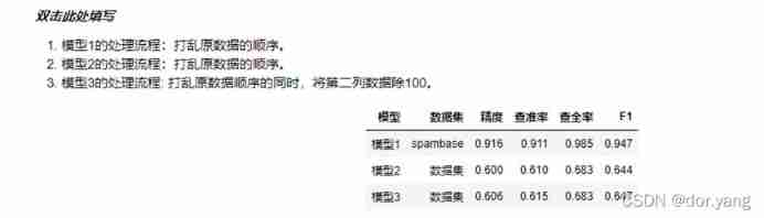
- experiment 3 Log probability regression completes the spam classification problem and Dota2 Prediction of results , Passing accuracy (accuracy), Precision rate (precision), Recall rate (recall),F1 Value to evaluate the prediction results .
- experiment 4 Linear discriminant analysis completes the spam classification problem and Dota2 Prediction of results , Try to transform the feature 、 Screening 、 After combination , Train the model and calculate the four indicators after ten fold cross validation :
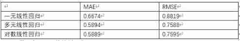
experiment 5 Use univariate linear regression 、 Multiple linear regression 、 Log linear regression and other linear regression models and log probability regression 、 Linear discriminant analysis predicts wine quality , Calculate the accuracy of ten fold cross validation . The experimental result is :
linear regression model :
Log probability regression , Linear discriminant analysis :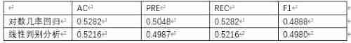
It can be found from the results that , In the linear regression model, the accuracy of multivariate linear regression and logarithmic linear regression is similar and better than that of univariate linear regression , The precision of log linear regression is better than that of linear discriminant analysis .
Evaluation criteria of results in the experiment :
precision (accuracy), Precision rate (precision), Recall rate (recall),F1 value ,MAE,RMSE
Standard description :
(1). Precision rate (Precision), Also called accuracy , The abbreviation means P. The accuracy rate is for our prediction results , It shows how many of the predicted positive samples are really positive samples .
(2). accuracy (Accuracy), The abbreviation means A. Accuracy is the proportion of the number of correctly classified samples to the total number of samples .Accuracy It reflects the ability of the classifier to judge the whole sample ( That is, positive can be determined as positive , Negative is judged to be negative ).
(3). Recall rate (Recall), Also called recall rate , The abbreviation means R. Recall is for our original sample , It shows how many positive examples in the sample are predicted correctly .
(4).F1 fraction (F1 Score), It is used to measure two categories in Statistics ( Or multi task two classification ) An indicator of model accuracy . It takes into account both the accuracy and recall of the classification model .F1 The score can be regarded as a weighted average of model accuracy and recall , Its maximum value is 1, The minimum is 0, A higher value means a better model .
(5).RMSE Is the root mean square error , It represents the difference between the predicted value and the observed value ( It's called residual error ) The sample standard deviation of . The root mean square error is to illustrate the dispersion of the sample . When doing nonlinear fitting ,RMSE The smaller the better. .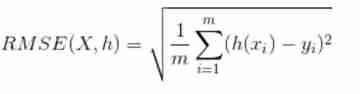
(6).MAE Is the mean absolute error , It represents the average of the absolute error between the predicted value and the observed value . It's a linear fraction , All individual differences are equally weighted on the average .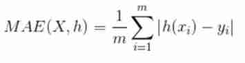
experimental analysis :
General form of linear model :
Vector form :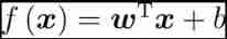
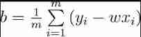
Minimize square error :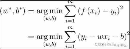
Respectively for ω and b Derivation , Available 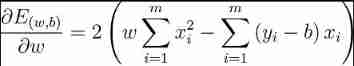
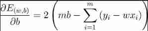
Make equal to 0, Get the closed form solution :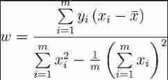
Experimental instructions :
Understanding of ten fold cross validation : Ten fold cross validation is to divide the data set into ten , Then take turns using nine of them as training sets , The rest is a test set . In the end 10 The predicted values are spliced and returned . Use this method , You can make full use of all the data in the data set , Thus, the occurrence of over fitting can be reduced to a certain extent .
2. Decision tree
Experimental content and some experimental results :
- experiment 1 Use the decision tree to complete DOTA2 Prediction of competition results , And draw the maximum depth 1-10 The change diagram of the accuracy of the ten fold cross validation of the decision tree , Choose to do questions by adjusting parameters , Get the model with the best generalization ability .
Considering the running time of the code ( Basically, it takes about twoorthree minutes for each parameter combination to build a tree ), In the code, set a larger step for each parameter list list , After building the tree with different parameters, analyze the performance and output the best results .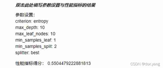
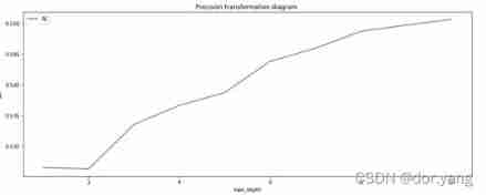
- experiment 2 Use sklearn.tree.DecisionTreeRegressor complete kaggle House price forecast , And draw the maximum depth from 1 To 30, The decision tree is on the training set and the test set MAE The curve of change .
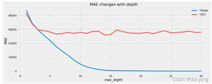
according to MAE chart , We choose a maximum depth of 15, Because when the maximum depth is less than 15 when ,MAE Rapid descent , When the maximum depth is greater than 10 after ,MAE Basically no change , Therefore, we choose the maximum depth of 15
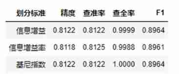
experiment 3 Use information gain , Information gain rate , The Gini index completes the decision tree , And calculate the maximum depth as 6 The accuracy of decision-making in training set and test set , Precision rate , Recall rate , F1 value .
experiment 4 Pre pruning using information gain rate division , Calculate the precision of decision tree with and without pre pruning , Precision rate , Recall and F1 value .
The process of pre pruning is after selecting an optimal feature each time , According to the selected classification criteria , Judge whether the accuracy after division is higher than that without division . Only in the case of higher accuracy after division, will we continue to recurse down , Otherwise, set the current node as a leaf node and take the class with the largest number of samples of the current node as the result .
in other words , The process of pre pruning , In the process of creating the decision tree, a pre pruning decision condition is added as the termination condition of the recursive program : If the current node is divided , The generalization ability of the model has not been improved , No division .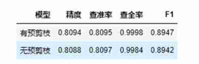
experiment 5 Realize the decision tree with post pruning , Compare the difference between pruning and non pruning in any data set .
In fact, pruning after implementation should be the same as experiment 3 , Build a common decision tree . And then the whole decision tree from bottom to top , Consider whether each node directly as a leaf will have better accuracy , If you have better accuracy, turn this node directly into leaves for pruning .
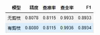
According to the model results we tested , We can see that the model with pruning has improved in all indicators , Just because the depth of our tree is 6 Promotion is not obvious
Explanation of relevant concepts of experiment :
1. Information gain :
The information gain is :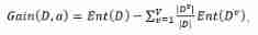
The information entropy is :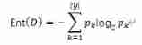
Information gain is the difference between the information entropy of the current node and the information entropy synthesis of all child nodes . The sum of the information entropy of all sub nodes is the weighted average of the information entropy of each sub node .
2. Information gain rate
The information gain rate is :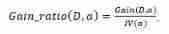
among :
IV(a) It can be regarded as taking the proportion of the size of the child node set to the current node set as information to calculate an information entropy , And as a penalty , When child nodes are also scattered , The greater the value of this penalty item .
3. gini index
The Gini value is :
attribute a The Gini value of :
Gini index is used to measure data D The purity of , The smaller the value of Gini index, the higher the purity of the data . attribute a The Gini value of is based on the attribute a Divide , The Gini values of child nodes are weighted average according to the size of the set .
Experimental analysis and summary :
“ prune ” It's decision tree learning algorithm “ Over fitting ” The primary means , Pre pruning can pass “ prune ” To avoid too many branches of decision-making , As a result, some characteristics of the training set itself are regarded as the general properties of all data , At the same time, it significantly reduces the training time and testing time
But pre pruning also brings the risk of under fitting , The current partition of some branches can't improve the generalization performance , However, the subsequent division based on it may lead to significant performance improvement . Pre pruning is based on “ greedy ” The essence forbids these branches to expand , It brings the risk of under fitting .
Then pruning technology because the bottom-up investigation and pruning are carried out after the decision-making training strategy tree is completed , Therefore, while obtaining greater generalization performance, it also pays the price of more overhead time .
3. neural network
Experimental content and some experimental results :
- experiment 1 Use sklearn The self-contained handwritten numeral data set completes the task of handwritten numeral classification , Draw the learning rate as 3,1,0.1,0.01 The change curve of the loss function of the training set
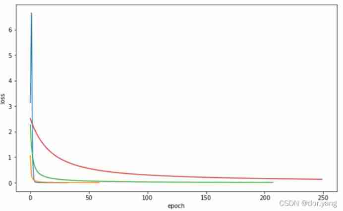
From the image we can see , When parameters learning_rate_init When the setting is large , Its training effect will produce great fluctuations ; And on the whole , The lower the learning rate ,loss What is needed to achieve convergence epoch The more , That is, the longer the training time , So that learning_rate_init=0.01,max_iter = 250 Under the condition of parameter setting ,loss Convergence is not achieved , Therefore, its accuracy is also lower than other models .
- experiment 2 Solving linear regression using gradient descent , Understand the effect of standardized treatment
After following the prompts to complete the code and start running , By printing the loss information, we can see that the loss value continues to rise , This is because of our raw data X Without proper treatment , Directly thrown into the neural network for training , As a result, when calculating the gradient , because X The order of magnitude is too large , This leads to an order of magnitude increase in the gradient , When the parameter is updated, the order of magnitude of the parameter keeps rising , As a result, the parameters cannot converge .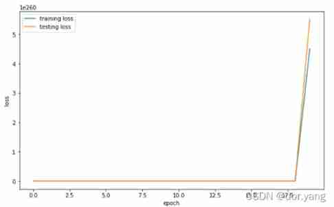
Normalize the parameters , Standardize it , Make the mean 0, Zoom to [−1,1] Re train the model after getting close :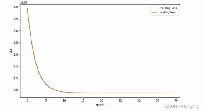
Calculate... On the test set MSE by :3636795867.3535
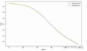
- experiment 3 Complete logarithmic probability regression , Use gradient descent to solve model parameters , Draw the change curve of the loss value of the model , Adjust learning rate and iteration rounds , Observe the change of loss value curve , According to the given learning rate and iteration rounds , Initialize new parameters , Draw the change curve of the loss value of the new model on the training set and the test set , Complete the accuracy filling in the form
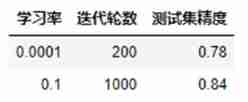
Through observation, it can be found that due to 0.0001 The learning rate is too low , Resulting in too slow convergence ,loss The curve of is even locally amplified into a linear change . and 0.1 The learning rate is better , When training to 200 It has begun to converge around the wheel . Therefore, if a larger learning rate is selected during training, the training rounds can be appropriately reduced , And when the learning rate is small , It is necessary to appropriately increase the training rounds .
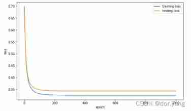
experiment 4 Implement a three-tier perceptron , Classify handwritten digital data sets , Draw the loss value change curve , complete kaggle MNIST Handwritten numeral classification task , According to the given hyperparametric training model , Complete the form
According to the requirements of the experiment , Adjust the parameters for training and evaluate the results :
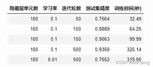
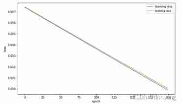
The data of the first four rows in the table is only different in the number of iteration rounds , Therefore, through observation, the learning rate is 0.1, The iteration rounds are 500 The graph of can be found , The model is in the process of training ,loss from 100 The rounds begin to converge gradually , In the test set and training set loss stay 200 The wheels are separated from each other , That is, there is a certain over fitting . Therefore, in the first four rows of data in the table , You can see that with the increase of iteration rounds , Accuracy is rising .
When the learning rate is set to 0.01 after , Because the update step is too small , So it can be found that although the iteration rounds are set to 500, Trained loss Still not converging , Therefore, the precision is not very good .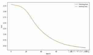
Experimental analysis and summary :
Comparative experiments 1 Different curves can be seen , When training, you need to choose an appropriate learning rate , The learning rate controls the update step size in the iterative process of the algorithm , If the learning rate is too high , It is not easy to converge , If too small , The convergence speed is easy to be too slow .
By experiment 3 You can find , When the learning rate is low , The accuracy of the model is low , And the loss value decreases linearly with the increase of iteration rounds . When the learning rate is high , The accuracy of the model is high , And the loss value will rapidly decrease in a very short period of iteration rounds , Later, as the number of iteration rounds increases, the reduction is not very obvious . Compare the two , We know , In model training , We can appropriately improve the learning rate , Reduce the number of iterations to achieve high-speed and high accuracy model training . The same is true in experiments 4 It is also shown in the experiment of , Because the learning rate is low , Lead to slow convergence , stay 500 There is still no convergence after iteration , This leads to lower accuracy .
边栏推荐
- The phenomenology of crypto world: Pioneer entropy
- 【LeetCode】501. Mode in binary search tree (2 wrong questions)
- Problem solving: attributeerror: 'nonetype' object has no attribute 'append‘
- Idea inheritance relationship
- The perfect car for successful people: BMW X7! Superior performance, excellent comfort and safety
- 1.五层网络模型
- LeetCode --- 1071. Great common divisor of strings problem solving Report
- How to make OS X read bash_ Profile instead of Profile file - how to make OS X to read bash_ profile not . profile file
- openresty ngx_lua变量操作
- 8. Commodity management - commodity classification
猜你喜欢
Master Fur

The perfect car for successful people: BMW X7! Superior performance, excellent comfort and safety

Zabbix
![ASP. Net core 6 framework unveiling example demonstration [01]: initial programming experience](/img/22/08617736a8b943bc9c254aac60c8cb.jpg)
ASP. Net core 6 framework unveiling example demonstration [01]: initial programming experience
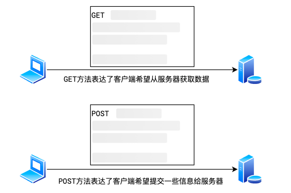
2.常见的请求方法
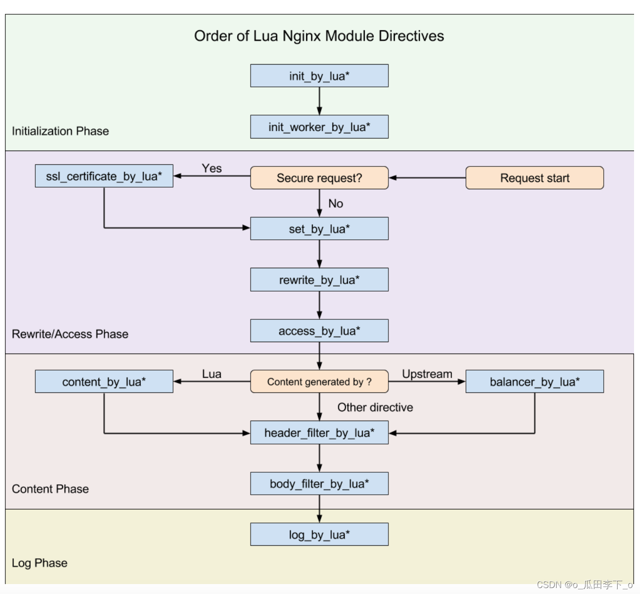
openresty ngx_ Lua execution phase
The perfect car for successful people: BMW X7! Superior performance, excellent comfort and safety
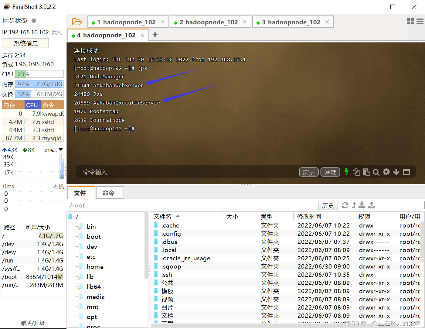
Azkaban installation and deployment
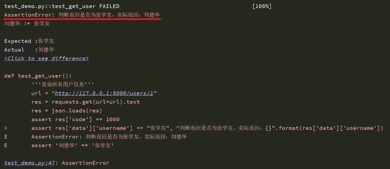
Pytest (5) - assertion
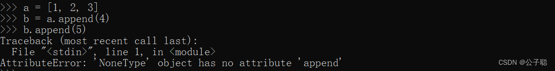
问题解决:AttributeError: ‘NoneType‘ object has no attribute ‘append‘
随机推荐
Last week's hot review (2.7-2.13)
Why are there fewer and fewer good products produced by big Internet companies such as Tencent and Alibaba?
College Students' innovation project management system
Why is this an undefined behavior- Why is this an undefined behavior?
Sqoop command
Use UDP to send a JPEG image, and UPD will convert it into the mat format of OpenCV after receiving it
Avoid material "minefields"! Play with super high conversion rate
Why do you understand a16z? Those who prefer Web3.0 Privacy Infrastructure: nym
2. Common request methods
【LeetCode】106. Construct binary tree from middle order and post order traversal sequence (wrong question 2)
D3js notes
GFS distributed file system
100 basic multiple choice questions of C language (with answers) 04
Zabbix
Privatization lightweight continuous integration deployment scheme -- 01 environment configuration (Part 1)
8. Commodity management - commodity classification
[daily problem insight] Li Kou - the 280th weekly match (I really didn't know it could be so simple to solve other people's problems)
ELK日志分析系统
Pat class a 1162 postfix expression
When to catch an exception and when to throw an exception- When to catch the Exception vs When to throw the Exceptions?