Machine learning plant leaf recognition

Identification of plant leaves ： Give the data set of blades ” Leaf shape .csv”, Describe the edges of plant leaves 、 shape 、 The numerical variables of these three features of texture have 64 individual （ common 64*3=192 A variable ）. Besides , also 1 Taxonomic variables recording the plant species to which each leaf belongs , common 193 A variable . Please use the feature selection method for feature selection , And compare the similarities and differences of the feature selection results （20 branch ）. Through data modeling , Complete the recognition of blade shape （30 branch ）.

Catalog

Catalog

Ideas

1 Import package

 2 Draw the correlation matrix （ According to the correlation matrix , Select features for Feature Engineering ）

3 Conduct PCA Dimension reduction

4 KNN Grid search optimization ,PCA Before and after

5 SVC

6. Logical regression

 

 

---

 

 

Ideas

1. Data analysis   visualization
2. establish Feature Engineering （ According to the correlation matrix , Select features for Feature Engineering . Including data preprocessing , Supplement missing values , Normalized data, etc ）
3. Machine learning algorithm Model to verify the analysis

 

 

1 Import package

import pandas as pd
from sklearn import svm
import numpy as np
from sklearn.svm import SVC
from sklearn.metrics import accuracy_score
from sklearn.model_selection import train_test_split
from sklearn.preprocessing import StandardScaler
from sklearn.decomposition import PCA

 

 2 Draw correlation matrix （ According to the correlation matrix , Select features for Feature Engineering ）

 

Train= pd.read_csv(" Leaf shape .csv")
X = Train.drop(['species'], axis=1)
Y = Train['species']

  

 

 

Train['species'].replace(map_dic.keys(), map_dic.values(), inplace=True)
Train.drop(['id'], inplace = True, axis = 1)
Train_ture = Train['species']
# Draw the correlation matrix 
corr = Train.corr()
f, ax = plt.subplots(figsize=(25, 25))
cmap = sns.diverging_palette(220, 10, as_cmap=True)
sns.heatmap(corr, cmap=cmap, vmax=.3, center=0,
            square=True, linewidths=.5)
plt.show()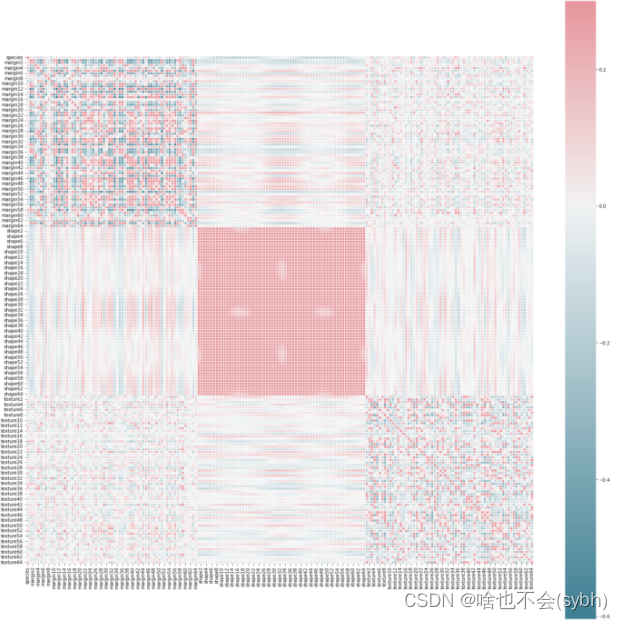

Supplement missing values

np.all(np.any(pd.isnull(Train)))

#false

                                                                                        

Training set test set division （80% Training set 、20% Test set ）

x_train,x_test,y_train,y_test=train_test_split(X,Y,test_size=0.2,random_state=123)

Normalize the data

standerScaler = StandardScaler()
x_train = standerScaler.fit_transform(x_train)
x_test = standerScaler.fit_transform(x_test)

 

 

3 Conduct PCA Dimension reduction

pca = PCA(n_components=0.9)
x_train_1 = pca.fit_transform(x_train)
x_test_1 = pca.transform(x_test)

## 44 Features 

 

 

4 KNN grid Search optimization ,PCA Before and after

from sklearn.neighbors import KNeighborsClassifier

knn_clf0 = KNeighborsClassifier()
knn_clf0.fit(x_train, y_train)
print('KNeighborsClassifier')

y_predict = knn_clf0.predict(x_test)
score = accuracy_score(y_test, y_predict)
print("Accuracy: {:.4%}".format(score))

print("PCA after ")

knn_clf1 = KNeighborsClassifier()
knn_clf1.fit(x_train_1, y_train)
print('KNeighborsClassifier')

y_predict = knn_clf1.predict(x_test_1)
score = accuracy_score(y_test, y_predict)
print("Accuracy: {:.4%}".format(score))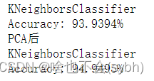

 

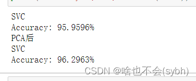
5 SVC

svc_clf = SVC(probability=True)
svc_clf.fit(x_train, y_train)

print("*"*30)
print('SVC')

y_predict = svc_clf.predict(x_test)
score = accuracy_score(y_test, y_predict)
print("Accuracy: {:.4%}".format(score))



svc_clf1 = SVC(probability=True)
svc_clf1.fit(x_train_1, y_train)

print("*"*30)
print('SVC')

y_predict1 = svc_clf1.predict(x_test_1)
score = accuracy_score(y_test, y_predict1)
print("Accuracy: {:.4%}".format(score))

 

 

6. Logical regression

from sklearn.linear_model import LogisticRegressionCV

lr = LogisticRegressionCV(multi_class="ovr", 
                          fit_intercept=True, 
                          Cs=np.logspace(-2,2,20), 
                          cv=2, 
                          penalty="l2", 
                          solver="lbfgs", 
                          tol=0.01)

lr.fit(x_train,y_train)
print(' Logical regression ')

y_predict = lr.predict(x_test)
score = accuracy_score(y_test, y_predict)
print("Accuracy: {:.4%}".format(score))

 

 

 

 

The accuracy of logistic regression is the highest 98.65

After feature selection and principal component analysis, the accuracy will not necessarily be improved