当前位置:网站首页>[pytorch practice] use pytorch to realize image style migration based on neural network
[pytorch practice] use pytorch to realize image style migration based on neural network
2022-07-07 12:33:00 【Sickle leek】
use PyTorch Realize image style migration based on Neural Network
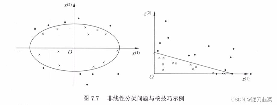
Style transfer , Also known as style transformation . Just give the original picture , And choose the artist's style pictures , You can convert the original picture into a picture with the corresponding artist style . The style transfer of images starts from 2015 year Gatys The paper of “Image Style Transfer Using Convolutional Neural Networks”, What we do is to fuse a content image with a style image , Get the composite image after style rendering . Examples are as follows : 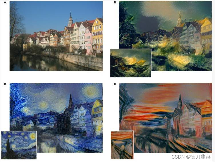
1. Introduction to the principle of style transfer
There are two types of pictures in style transfer : One is Style picture , It's usually the work of some artists , Often with obvious artist style , Including color 、 line 、 Outline, etc ; The other is Content picture , These pictures often come from the real world , Such as personal photography . Using style migration, we can convert content pictures into artist style pictures .
Gatys The method proposed by et al. Is called Neural Style, But their implementation is too complicated .Justin Johnson Et al. Proposed an algorithm to quickly realize style migration , be called Fast Neural Style. When used Fast Neural Style After training a style model , Usually it's just GPU Run for a few seconds , The corresponding style transfer effect can be generated .
Fast Neural Style and Neural Style There are mainly the following two differences :
(1)Fast Neural Style Train a model for each style image , Then it can be used repeatedly , Fast style migration .Neural Style No special training model is required , Just constantly adjust the pixel value of the image from the noise , The guidance finally gets the structure , Slower , It takes more than ten minutes to dozens of minutes .
(2) It is generally believed that Neural Style The effect of the generated image will be better than Fast Neural Style The effect is good .
Here we mainly introduce Fast Neural Style The implementation of the .
To produce realistic style migration pictures , There are two requirements :
- The image to be generated is in the content 、 The details should be similar to the input content image as much as possible ;
- The image to be generated is similar to the style image as much as possible .
Accordingly , Define two losses content loss and style loss, Used to measure the above two indicators .
- content loss The commonly used method is to calculate the difference per pixel , also called pixel-wise loss, The difference between the generated image and the original image per pixel should be as small as possible . But this method has many irrationalities ,Justin A better calculation is proposed content loss Methods , be called perceptual loss. differ pixel-wise loss Calculate the difference at the pixel level ,perceptual loss What we calculate is the difference of images at a higher semantic level . Use the upper layer of the pre trained neural network as the perceptual feature of the picture , Then calculate the difference between the two as perceptual loss.
During style transfer , The pixels of the generated image are not required to be the same as each pixel in the original image , The pursuit is that the generated image has the same characteristics as the original image .
In general use Gram matrix To represent the style characteristics of the image . For every picture , The output shape of the convolution layer is C × H × W C\times H\times W C×H×W,C Is the number of channels of convolution kernel , It is generally called having C Convolution kernels , Each convolution kernel learns different features of the image . The output of each convolution kernel H × W H\times W H×W One representing this image feature map, It can be considered as a special image —— The original color image can be regarded as RGB Three feature map Special stitching feature map. By calculating each feature map Similarity between , You can get the style characteristics of the image . For one C × H × W C\times H\times W C×H×W Of feature maps F F F,Gram Matrix The shape of is C × C C\times C C×C, Its first i , j i,j i,j Elements G i , j G_{i,j} Gi,j The calculation of is as follows :
G i , j = ∑ k F i k F j k G_{i,j}=\sum_{k}F_{ik}F_{jk} Gi,j=k∑FikFjk
among F i k F_{ik} Fik On behalf of the i individual feature map Of the k Pixels .
It should be noted that :
- Gram Matrix The calculation of adopts the form of accumulation , Abandoning spatial information .
- Gram Matrix The result of feature maps F Regardless of the scale of , Only related to the number of channels . No matter what H,W What's the size of , Last Gram Matrix All shapes are C×C.
- For one C × H × W C\times H\times W C×H×W Of feature maps, It can be quickly calculated by adjusting the shape and matrix multiplication Gram Matrix, That will be first F Adjusted for C × ( H W ) C\times (HW) C×(HW) Two dimensional matrix of , And then calculate F ⋅ F T F\cdot F^T F⋅FT, The result is Gram Matrix.
Practice has proved the use of Gram Matrix The style characteristics of the image are transferred in style 、 Excellent performance in tasks such as texture synthesis . All in all :
- The high-level output of neural network can be used as the perceptual feature description of image
- High level output of neural network Gram Matrix It can be used as the style feature description of the image .
- The goal of style transfer is to make the perceptual characteristics of the generated image and the original image as similar as possible , And the style characteristics of style pictures are as similar as possible .
2. Fast Neural Style Network structure
Fast Neural Style It specifically involves a network for style migration , Input the original picture , The network will automatically generate the target image . As shown in the figure below :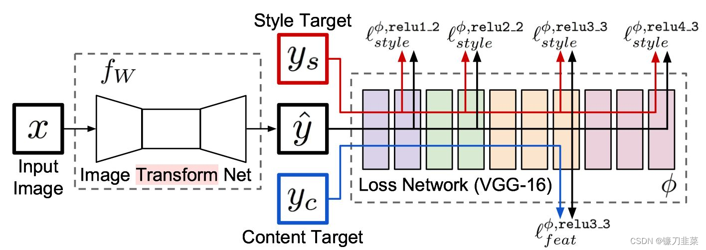
The whole network is composed of two parts :Image transformation network、 Loss Netwrok;
- Image Transformation network It's a deep residual conv netwrok, Used to input image (content image) direct transform With style Image ;
- and loss network Parameter is fixed Of , there loss network and A Neural Algorithm of Artistic Style The network structure in is consistent , Just don't update the parameters (neural style Of weight It 's also constant , The difference is pixel level loss and per loss The difference between ,neural style Inside is the update pixel , Get the final composite photo ), It's just for content loss and style loss The calculation of , This is what we call perceptual loss,
One is the network that generates pictures , It's the one in front of the picture , Mainly used to generate pictures , Behind it is a VGG The Internet , Mainly feature extraction , In fact, these characteristics are used to calculate the loss , When we train, we only train the front network , The later use is based on ImageNet Trained models , Do feature extraction directly .
As shown in the figure above , x x x It's the input image , In the task of style transfer y c = x y_c=x yc=x, y s y_s ys It's a style picture ,Image Transform Net f W f_W fW It is the style migration network we are involved in , Image for input x x x, Can return a new image y ^ \hat{y} y^, y ^ \hat{y} y^ In terms of image content, it is similar to y c y_c yc be similar , But in style, it is different from y s y_s ys be similar . Loss network (loss network) No training , It is only used to calculate perceptual characteristics and style characteristics . Loss network adopts ImageNet It's pre trained VGG-16.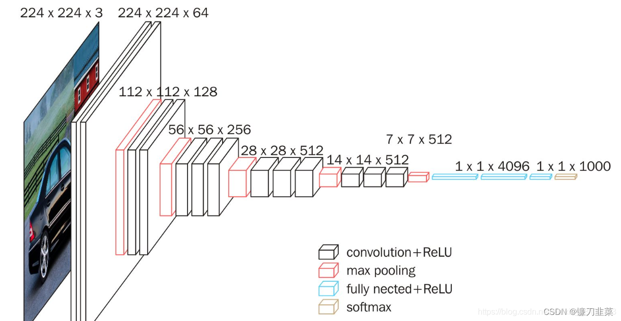
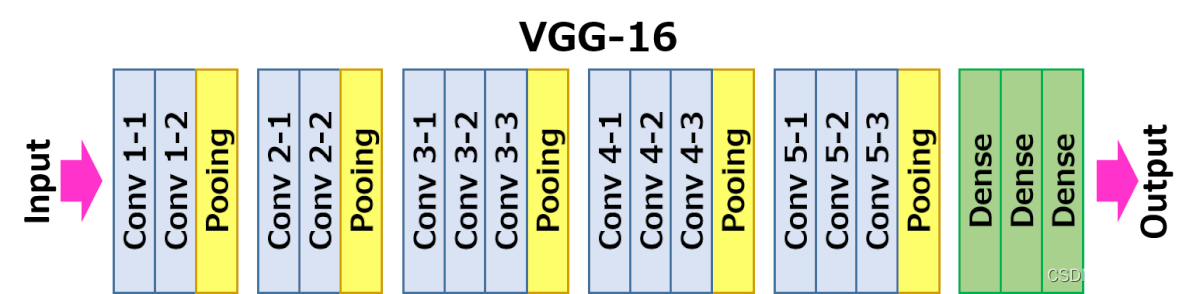
Network from left to right 5 Convolution blocks , Two convolution blocks pass through MaxPooling Layer differentiation , Each convolution block has 2~3 Convolution layers , Each convolution layer is followed by ReLU Activate once . among relu2_2 It means the first one 2 The th of convolution block 2 The active layer of a convolution layer (ReLU) Output .
Fast Neural Style The training steps are as follows :
(1) Enter a picture x To f W f_W fW in , Get the results y ^ \hat{y} y^;
(2) take y ^ \hat{y} y^ and y c y_c yc( In fact, that is x) Input to loss network(VGG-16) in , Calculate where it is relu3_3 Output , And calculate the mean square error between them as content loss.
(3) take y ^ \hat{y} y^ and y s y_s ys( Style picture ) Input to loss network in , Calculate where it is relu1_2,relu2_2,relu3_3 and relu4_3 Output , Then calculate their Gram Matrix The mean square error of is taken as style loss.
(4) The two losses add up , And back propagation . to update f W f_W fW Parameters of , Fix loss network Immobility .
(5) Jump back to the first step , Keep training f W f_W fW.
First understand the structure of the full convolution network . The input is a picture , The output is also a picture , This kind of network is generally implemented as a network structure with all convolution layers but no all connection layers . For the convolution layer , When the input feature map( Or pictures ) The size is C i n × H i n × W i n C_{in}\times H_{in}\times W_{in} Cin×Hin×Win, The convolution kernel has C o u t C_{out} Cout individual , The size of the convolution kernel is K K K,padding The size is P P P、 In steps of S S S when , Output feature maps The shape of is C o u t × H o u t × W o u t C_{out}\times H_{out}\times W_{out} Cout×Hout×Wout, among
H o u t = f l o o r ( H i n + 2 ∗ P − K ) / S + 1 H_{out}=floor(H_{in}+2\ast P-K)/S+1 Hout=floor(Hin+2∗P−K)/S+1
W o u t = f l o o r ( W i n + 2 ∗ P − K ) / S + 1 W_{out}=floor(W_{in}+2\ast P-K)/S+1 Wout=floor(Win+2∗P−K)/S+1
If the size of the input picture is 3×256×256, The convolution kernel size of the first layer convolution is 3,padding by 1, In steps of 2, The number of channels is 128, So the output feature map shape , According to the above formula, the result is :
H o u t = f l o o r ( 256 + 2 ∗ 1 − 3 ) / 2 + 1 = 128 H_{out} = floor(256+2\ast 1-3)/2+1=128 Hout=floor(256+2∗1−3)/2+1=128
W o u t = f l o o r ( 256 + 2 ∗ 1 − 3 ) / 2 + 1 = 128 W_{out} =floor(256+2\ast 1-3)/2+1=128 Wout=floor(256+2∗1−3)/2+1=128
So the final output is C o u t × H o u t × W o u t = 128 × 128 × 128 C_{out}\times H_{out}\times W_{out}=128\times 128\times 128 Cout×Hout×Wout=128×128×128, That is, the scale is reduced by half , The number of channels increases . If the step size is changed from 2 Change to 1, Then the output shape is 128×256×256, That is, the scale remains unchanged , Only the number of channels increases .
In addition to the convolution layer , There's another one called Transpose the convolution layer (Transposed Convolution), Some people call it deconvolution (DeConvolution), It can be simply regarded as the inverse operation of convolution . For the convolution operation , When the step length is greater than 1 when , It performs operations similar to down sampling , And for transpose convolution , When the step length is greater than 1 when , It performs operations similar to upsampling . An important advantage of full convolution networks is that there is no requirement for the size of the input , In this way, images with different resolutions can be accepted when style migration .
The style transfer structure mentioned in the paper is all composed of convolution 、Batch Normalization And activation layer , Does not include the full connection layer , We don't use Batch Normalization, In its place Instance Normalization.
Instance Normalization and Batch Normalization The only difference is InstaneNorm Only calculate the mean and variance of each sample , and BatchNorm Will be to a batch Find the mean value of all samples in .
 For example, for a B×C×H×W Of tensor, stay Batch Normalization When calculating the mean in , Will calculate B×H×W The mean of the number , share C A mean , and Instance Normalization Calculation H×W The mean of the number , The total of B×C A mean .
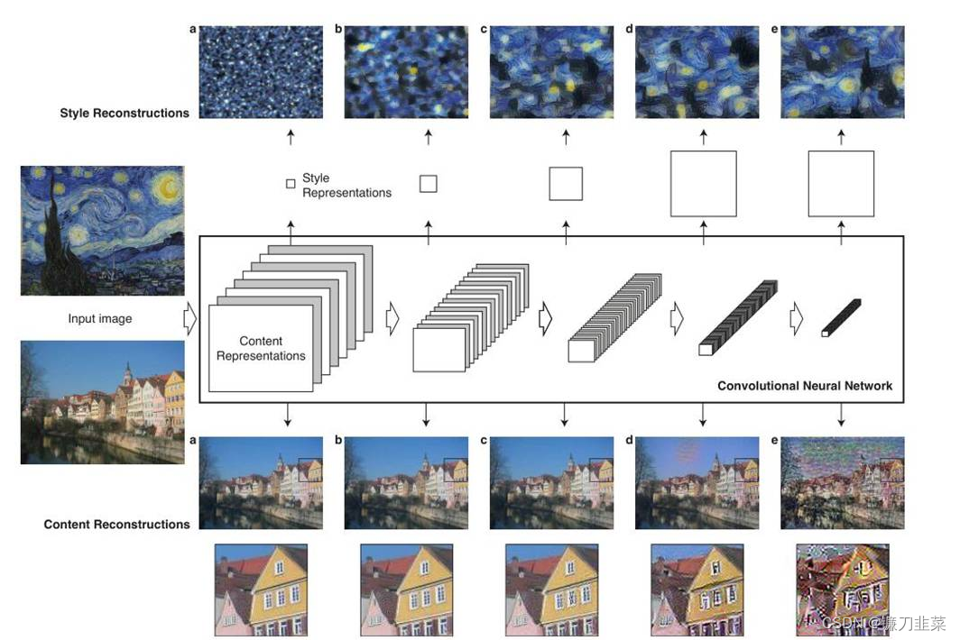
As shown in the figure above , The two pictures on the far left (input image) One is input as content , One is input as style , Go through separately VGG16 Of 5 individual block, It can be seen from the shallow and deep , The resulting feature map (feature map) The height and width of gradually decrease , But the depth is gradually increasing ,Gatys In order to let people see each more intuitively block Extracted features , So I made a trick, namely Feature reconstruction , The extracted features are visualized . But you can see that ,** To a large extent, the extraction of content image features preserves the information of the original image , But for style pictures , Basically, I can't see the appearance of the original picture , It can be roughly considered that the extracted style . Why is that ?** It turns out that the feature extraction processing for these two images is different , You can see in the next picture .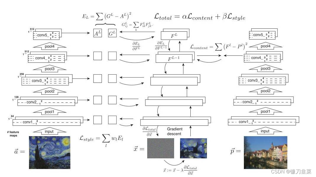
The pictures on both sides are style pictures , Write it down as a → \overrightarrow{a} a, And content pictures p → \overrightarrow{p} p, At the same time, we also need a third randomly generated noise picture , You need to iterate over noisy images constantly , Until you get a composite picture that combines content and style . Content picture p → \overrightarrow{p} p after VGG16 Online 5 individual block You will get feature map, Write it down as P l P^l Pl, That is to say l individual block The resulting features , Noise picture x → \overrightarrow{x} x after VGG16 Online 5 individual block The obtained characteristic map is marked as F l F^l Fl.
For content loss , Take only Conv4_2 Characteristics of the layer , Calculate the Euclidean distance between content image features and noise image features , Formula for :
L c o n t e n t ( p → , x → , l ) = 1 2 ∑ i , j ( F i j l − P i j l ) 2 \mathcal{L}_{content}(\overrightarrow{p},\overrightarrow{x}, l)=\frac{1}{2}\sum_{i,j}(F_{ij}^l-P_{ij}^l)^2 Lcontent(p,x,l)=21i,j∑(Fijl−Pijl)2
Loss of style , The calculation method is somewhat different . According to the above known , Noise picture x → \overrightarrow{x} x after VGG16 Online 5 individual block The obtained characteristics are recorded as F l F^l Fl, F l F^l Fl Of gram The matrix is written as G l G^l Gl, Style picture a → \overrightarrow{a} a The resulting feature map , Calculate again gram The content obtained after the matrix is recorded as A l A^l Al, Calculated after G l G^l Gl and A l A^l Al European distance between , among gram The formula of the matrix is :
KaTeX parse error: Can't use function '$' in math mode at position 9: G_{ij}^l$̲=\sum_k F_{ik}^…
The formula of style loss is :
E l = 1 4 N l 2 M l 2 ∑ i , j ( G i j l − A i j l ) 2 E_l=\frac{1}{4N_l^2M_l^2}\sum_{i,j}(G_{ij}^l-A_{ij}^l)^2 El=4Nl2Ml21i,j∑(Gijl−Aijl)2
The coefficient before the formula is a standardized operation , That is, divide by the square of the area .
It should be noted that , When calculating style loss ,5 individual block The extracted features are used to calculate , When calculating content loss , Actually, only the fourth one is used block Extracted features . This is because of each block The extracted style features are different , Participation in computing can increase the diversity of styles , And each of the content pictures block The extracted features have little difference , So just take one .
The total loss is the linear sum of content loss and style loss , change α and β The proportion of content and style can be adjusted .
L t o t a l ( p → , a → , x → ) = α L c o n t e n t ( p → , x → ) + β L s t y l e ( a → , x → ) \mathcal{L}_{total}(\overrightarrow{p}, \overrightarrow{a}, \overrightarrow{x})=\alpha \mathcal{L}_{content}(\overrightarrow{p}, \overrightarrow{x})+\beta \mathcal{L}_{style}(\overrightarrow{a}, \overrightarrow{x}) Ltotal(p,a,x)=αLcontent(p,x)+βLstyle(a,x)
The code also uses a trick, total loss We will add a total variation loss Used to reduce noise , Make the composite image look smoother .
The last thing to note is this ,Gatys Calculated total loss It's a noise picture x → \overrightarrow{x} x Finding partial derivatives , and Johnson Calculated loss Is the weight of the custom network w Finding partial derivatives .
3. use PyTorch Achieve style migration
Dataset download address :https://pjreddie.com/projects/coco-mirror/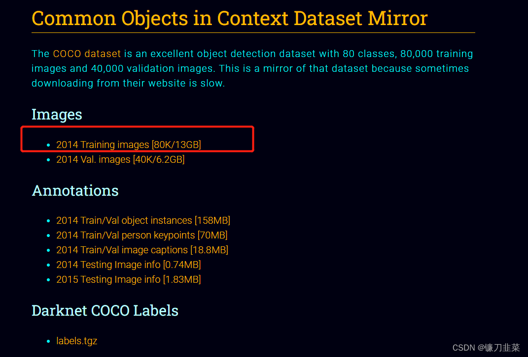
3.1 First look at how to use pre training VGG.
class Vgg16(nn.Module):
    def __init__(self, requires_grad=False):
        super(Vgg16, self).__init__()
        vgg_pretrained_ft = vgg16(pretrained=False)
        vgg_pretrained_ft.load_state_dict(torch.load("vgg16-397923af.pth"))
        vgg_pretrained_features = nn.Sequential(*list(vgg_pretrained_ft.features.children()))
        self.slice1 = nn.Sequential()
        self.slice2 = nn.Sequential()
        self.slice3 = nn.Sequential()
        self.slice4 = nn.Sequential()

        for x in range(4):
            self.slice1.add_module(str(x), vgg_pretrained_features[x])
        for x in range(4, 9):
            self.slice2.add_module(str(x), vgg_pretrained_features[x])
        for x in range(9, 16):
            self.slice3.add_module(str(x), vgg_pretrained_features[x])
        for x in range(16, 23):
            self.slice4.add_module(str(x), vgg_pretrained_features[x])

        if not requires_grad:
            for param in self.parameters():
                param.requires_grad = False

    def forward(self, X):
        h = self.slice1(X)
        h_relu1_2 = h
        h = self.slice2(h)
        h_relu2_2 = h
        h = self.slice3(h)
        h_relu3_3 = h
        h = self.slice4(h)
        h_relu4_3 = h
        vgg_outputs = namedtuple('VggOutputs', ['relu1_2', 'relu2_2', 'relu3_3', 'relu4_3'])
        result = vgg_outputs(h_relu1_2, h_relu2_2, h_relu3_3, h_relu4_3)
        return result
In the style migration network , You need to get the output of the middle layer , Therefore, it is necessary to modify the forward propagation process of the network , Save the output of the corresponding layer . At the same time, there are many layers that do not need , It can be deleted to save content .
** stay torchvision in , VGG The implementation of consists of two nn.Sequential Object composition , One is features, Inclusion convolution 、 Activate and MaxPool layer , Used to extract image features ; The other is classifier, Including full connection , Used to classify .** Can pass vgg.features Directly obtain the corresponding nn.Sequential object . In this way, when propagating forward , After calculating the output of the specified layer , Save the results in a list in , And then use namedtuple Name binding , So that you can get through output.relu1_2 Access the first element , More convenient and intuitive . Of course, we can also use layer.register_forward_hook Get the output of the corresponding layer .
3.2 Next, we need to realize style migration network
Realize style migration network reference Pytorch An official example of , Its structure can be summarized as follows :
- First down sampling , Post up sampling , Reduce the amount of calculation
- Use the residual structure to make the network deeper
- The way of edge filling is no longer the traditional way of filling 0, Instead, a method called Reflection Pad Complement strategy : The pixels of the upper, lower, left and right reflection edges are complemented .
- Upsampling no longer uses traditional ConvTransposed2d, But first Upsample, And then use Conv2d, Do this to avoid Checkerboard Artifacts The phenomenon .
- Batch Normalization All changed Instance Normalization.
- There is no full connection layer in the network , Linear operation is convolution , Therefore, there is no requirement for the size of input and output .
For common network structures , It can be realized as nn.Module object , As a special layer . therefore , take Conv,UpConv And residual blocks are implemented as a special layer :
# -*- coding: utf-8 -*-#

# ----------------------------------------------
# Name: transformer_net.py
# Description:
# Author: PANG
# Date: 2022/6/27
# ----------------------------------------------
class ConvLayer(nn.Module):
    """ add ReflectionPad for Conv  The default convolution padding Operation is complement 0, Here we use boundary reflection filling  """

    def __init__(self, in_channels, out_channels, kernel_size, stride):
        super(ConvLayer, self).__init__()
        reflection_padding = int(np.floor(kernel_size / 2))
        self.reflection_pad = nn.ReflectionPad2d(reflection_padding)
        self.conv2d = nn.Conv2d(in_channels, out_channels, kernel_size, stride)

    def forward(self, x):
        out = self.reflection_pad(x)
        out = self.conv2d(out)
        return out


class UpsampleConvLayer(nn.Module):
    """  The default convolution padding Operation is complement 0, Here we use boundary reflection filling   Sample first , Then do a convolution (Conv2d), Instead of adopting ConvTranspose2d """

    def __init__(self, in_channels, out_channels, kernel_size, stride, upsample=None):
        super(UpsampleConvLayer, self).__init__()
        self.upsample = upsample
        reflection_padding = int(np.floor(kernel_size / 2))
        self.reflection_pad = nn.ReflectionPad2d(reflection_padding)
        self.conv2d = nn.Conv2d(in_channels, out_channels, kernel_size, stride)

    def forward(self, x):
        x_in = x
        if self.upsample:
            x_in = nn.functional.interpolate(x_in, mode='nearest', scale_factor=self.upsample)
        out = self.reflection_pad(x_in)
        out = self.conv2d(out)
        return out


class ResidualBlock(nn.Module):
    """ introduced in: https://arxiv.org/abs/1512.03385 recommended architecture: http://torch.ch/blog/2016/02/04/resnets.html """

    def __init__(self, channels):
        super(ResidualBlock, self).__init__()
        self.conv1 = ConvLayer(channels, channels, kernel_size=3, stride=1)
        self.in1 = nn.InstanceNorm2d(channels, affine=True)
        self.conv2 = ConvLayer(channels, channels, kernel_size=3, stride=1)
        self.in2 = nn.InstanceNorm2d(channels, affine=True)
        self.relu = nn.ReLU()

    def forward(self, x):
        residual = x
        out = self.relu(self.in1(self.conv1(x)))
        out = self.in2(self.conv2(out))
        out = out + residual
        return out


class TransformerNet(nn.Module):
    def __init__(self):
        super(TransformerNet, self).__init__()
        #  Lower convolution
        self.initial_layers = torch.nn.Sequential(
            ConvLayer(3, 32, kernel_size=9, stride=1),
            nn.InstanceNorm2d(32, affine=True),
            nn.ReLU(True),

            ConvLayer(32, 64, kernel_size=3, stride=2),
            torch.nn.InstanceNorm2d(64, affine=True),
            torch.nn.ReLU(True),

            ConvLayer(64, 128, kernel_size=3, stride=2),
            torch.nn.InstanceNorm2d(128, affine=True),
            torch.nn.ReLU(True)
        )

        # Residual layers( Residual layer )
        self.res_layers = torch.nn.Sequential(
            ResidualBlock(128),
            ResidualBlock(128),
            ResidualBlock(128),
            ResidualBlock(128),
            ResidualBlock(128)
        )

        # Upsampling layers( Upper sampling layer )
        self.upsample_layers = torch.nn.Sequential(
            UpsampleConvLayer(128, 64, kernel_size=3, stride=1, upsample=2),
            torch.nn.InstanceNorm2d(64, affine=True),
            torch.nn.ReLU(True),

            UpsampleConvLayer(64, 32, kernel_size=3, stride=1, upsample=2),
            torch.nn.InstanceNorm2d(32, affine=True),
            torch.nn.ReLU(True),

            ConvLayer(32, 3, kernel_size=9, stride=1)
        )

    def forward(self, X):
        y = self.initial_layers(X)
        y = self.res_layers(y)
        y = self.upsample_layers(y)
        return y
stay TransformerNet There are three parts in it : Down sampled convolution layer , Depth residual layer and up sampled convolution layer . It makes full use of nn.Sequential, To avoid the forward Write code repeatedly in .
After setting up the network , Need to implement some tool functions , for example gram_matrix.
from PIL import Image

IMAGENET_MEAN = [0.485, 0.456, 0.406]
IMAGENET_STD = [0.229, 0.224, 0.225]


def load_image(filename, size=None, scale=None):
    img = Image.open(filename).convert('RGB')
    if size is not None:
        img = img.resize((size, size), Image.ANTIALIAS)
    elif scale is not None:
        img = img.resize((int(img.size[0] / scale), int(img.size[1] / scale)), Image.ANTIALIAS)
    return img


def save_image(filename, data):
    img = data.clone().clamp(0, 255).numpy()
    img = img.transpose(1, 2, 0).astype('uint8')
    img = Image.fromarray(img)
    img.save(filename)


def gram_matrix(y):
    """  Enter shape b, c, h, w  Shape of the output b, c, c :param y: image :return: gram matrix """
    (b, ch, h, w) = y.size()
    features = y.view(b, ch, w * h)
    features_t = features.transpose(1, 2)
    gram = features.bmm(features_t) / (ch * h * w)
    return gram


def normal_batch(batch):
    """  Input : b, ch, h, w 0~255,  It's a Variable  Output : b, ch, h, w  about -2~2,  It's a Variable :param batch: :return: """
    mean = batch.new_tensor(IMAGENET_MEAN).view(-1, 1, 1)
    std = batch.new_tensor(IMAGENET_STD).view(-1, 1, 1)
    batch = batch.div_(255.0)
    return (batch - mean) / std
When the tools and functions of the above network definition are implemented , Started training the network .
def train(args):
    device = torch.device('cuda' if args.cuda else 'cpu')
    np.random.seed(args.seed)
    torch.manual_seed(args.seed)

    #  Data loading
    transform = transforms.Compose([
        transforms.Resize(args.image_size),
        transforms.CenterCrop(args.image_size),
        transforms.ToTensor(),
        transforms.Lambda(lambda x: x.mul(255))
    ])
    train_dataset = datasets.ImageFolder(args.dataset, transform)
    train_loader = DataLoader(train_dataset, batch_size=args.batch_size)
    #  convert to binary
    transformer = TransformerNet().to(device)
    optimizer = Adam(transformer.parameters(), args.lr)
    mse_loss = torch.nn.MSELoss()
    # VGG16
    vgg = Vgg16(requires_grad=False).to(device)
    #  Get the data of style pictures
    style_transform = transforms.Compose([
        transforms.ToTensor(),
        transforms.Lambda(lambda x: x.mul(255))
    ])
    style = utils.load_image(args.style_image, size=args.style_size)
    style = style_transform(style)
    style = style.repeat(args.batch_size, 1, 1, 1).to(device)

    feature_style = vgg(utils.normal_batch(style))
    gram_style = [utils.gram_matrix(y) for y in feature_style]

    for e in range(args.epochs):
        #  Training
        agg_content_loss = 0
        agg_style_loss = 0
        count = 0
        transformer.train()
        for batch_id, (x, _) in enumerate(train_loader):
            n_batch = len(x)
            count += n_batch
            optimizer.zero_grad()

            x = x.to(device)
            y = transformer(x)

            y = utils.normal_batch(y)
            x = utils.normal_batch(x)

            features_y = vgg(y)
            features_x = vgg(x)

            #  Calculation content_loss,  It's only used. relu2_2
            content_loss = args.content_weight * mse_loss(features_y.relu2_2, features_x.relu2_2)

            # style loss At the same time 4 Layer output
            style_loss = 0
            for ft_y, gm_s in zip(features_y, gram_style):
                gm_y = utils.gram_matrix(ft_y)
                style_loss += mse_loss(gm_y, gm_s[:n_batch, :, :])
            style_loss *= args.style_weight

            #  Back propagation , Update gradient , Only update here transformer Parameters of , Not updated VGG16 Of
            total_loss = content_loss + style_loss
            total_loss.backward()
            optimizer.step()

            #  Loss smoothing
            agg_content_loss += content_loss.item()
            agg_style_loss += style_loss.item()

            if (batch_id + 1) % args.log_interval == 0:
                mesg = "{}\tEpoch {}:\t[{}/{}]\tcontent: {:.6f}\tstyle: {:.6f}\ttotal: {:.6f}".format(
                    time.ctime(), e + 1, count, len(train_dataset),
                                  agg_content_loss / (batch_id + 1),
                                  agg_style_loss / (batch_id + 1),
                                  (agg_content_loss + agg_style_loss) / (batch_id + 1)
                )
                print(mesg)
            if args.checkpoint_model_dir is not None and (batch_id + 1) % args.checkpoint_interval == 0:
                transformer.eval().cpu()
                ckpt_model_filename = "ckpt_epoch_" + str(e) + "_batch_id_" + str(batch_id + 1) + ".pth"
                ckpt_model_path = os.path.join(args.checkpoint_model_dir, ckpt_model_filename)
                torch.save(transformer.state_dict(), ckpt_model_path)
                transformer.to(device).train()

    #  Save the model
    transformer.eval().cpu()
    save_model_filename = "epoch_" + str(args.epochs) + "_" + str(time.ctime()).replace(' ', '_') + "_" + str(
        args.content_weight) + "_" + str(args.style_weight) + ".model"
    save_model_path = os.path.join(args.save_model_dir, save_model_filename)
    torch.save(transformer.state_dict(), save_model_path)

    print("\nDone, trained model saved at", save_model_path)
The pictures used for training here are MS COCO 2014 training Data set of , It contains about 8 Ten thousand pictures ,13GB.
After training , To load the pre trained model and transfer the style of the specified image . The code is as follows :
def stylize(args):
    device = torch.device('cuda' if args.cuda else 'cpu')
    #  The image processing
    content_image = utils.load_image(args.content_image, scale=args.content_scale)
    content_transform = transforms.Compose([
        transforms.ToTensor(),
        transforms.Lambda(lambda x: x.mul(255))
    ])

    content_image = content_transform(content_image)
    content_image = content_image.unsqueeze(0)

    if args.model.endswith('.onnx'):
        output = stylize_onnx(content_image, args)
    else:
        with torch.no_grad():
            #  Model
            style_model = TransformerNet()
            state_dict = torch.load(args.model)
            # remove saved deprecated running_* keys in InstanceNorm from the checkpoint
            for k in list(state_dict.keys()):
                if re.search(r'in\d+\.running_(mean|var)$', k):
                    del state_dict[k]
            #  Style migration and preservation
            style_model.load_state_dict(state_dict).to(device).eval()
            if args.export_onnx:
                assert args.export_onnx.endswith('.onnx'), "Export model file should end with .onnx"
                output = torch.onnx._export(
                    style_model, content_image, args.export_onnx, opset_version=11
                ).cpu()
            else:
                output = style_model(content_image).cpu()
                utils.save_image(args.output_image, output[0])
Reference material
[1] Deep learning -VGG16 The principle,
[2] Advanced notes of machine learning II | In depth understanding of Neural Style
[3] NEURAL TRANSFER USING PYTORCH
[4] PyTorch The official sample
边栏推荐
- gcc 编译报错
- 免备案服务器会影响网站排名和权重吗?
- DOM parsing XML error: content is not allowed in Prolog
- The IDM server response shows that you do not have permission to download the solution tutorial
- BGP third experiment report
- Session
- 解密GD32 MCU产品家族,开发板该怎么选?
- Inverted index of ES underlying principle
- What is an esp/msr partition and how to create an esp/msr partition
- Tutorial on principles and applications of database system (010) -- exercises of conceptual model and data model
猜你喜欢
SQL Lab (46~53) (continuous update later) order by injection
【统计学习方法】学习笔记——支持向量机(下)
![[pytorch practice] image description -- let neural network read pictures and tell stories](/img/39/b2c61ae0668507f50426b01f2deee4.png)
[pytorch practice] image description -- let neural network read pictures and tell stories
Static comprehensive experiment
Attack and defense world - PWN learning notes
Completion report of communication software development and Application
About sqli lab less-15 using or instead of and parsing

On valuation model (II): PE index II - PE band

Xiaohongshu microservice framework and governance and other cloud native business architecture evolution cases
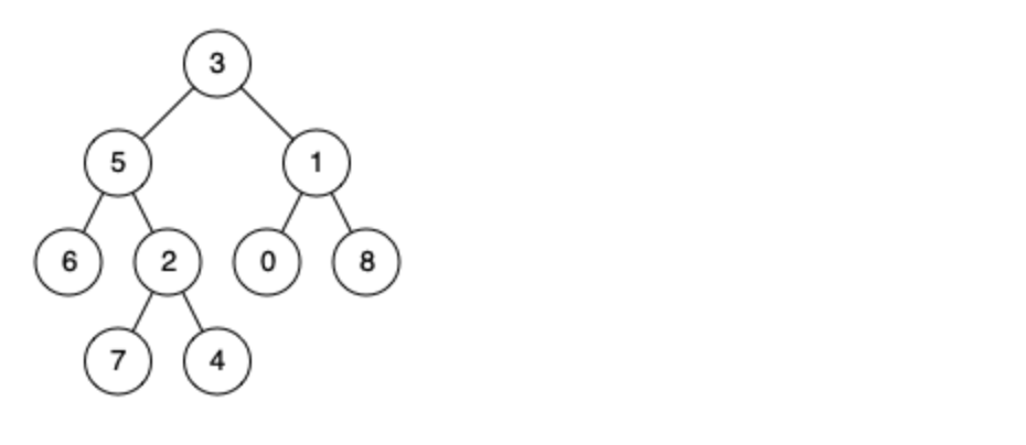
leetcode刷题:二叉树24(二叉树的最近公共祖先)
随机推荐
EPP+DIS学习之路(1)——Hello world!
平安证券手机行开户安全吗?
百度数字人度晓晓在线回应网友喊话 应战上海高考英语作文
leetcode刷题:二叉树20(二叉搜索树中的搜索)
Sort out the garbage collection of JVM, and don't involve high-quality things such as performance tuning for the time being
数据库系统原理与应用教程(007)—— 数据库相关概念
ES底层原理之倒排索引
对话PPIO联合创始人王闻宇:整合边缘算力资源,开拓更多音视频服务场景
2022-07-07日报:GAN发明者Ian Goodfellow正式加入DeepMind
Ctfhub -web SSRF summary (excluding fastcgi and redI) super detailed
Epp+dis learning road (2) -- blink! twinkle!
[statistical learning methods] learning notes - improvement methods
Sign up now | oar hacker marathon phase III midsummer debut, waiting for you to challenge
NGUI-UILabel
How much does it cost to develop a small program mall?
Tutorial on principles and applications of database system (010) -- exercises of conceptual model and data model
Cenos openssh upgrade to version 8.4
ENSP MPLS layer 3 dedicated line
leetcode刷题:二叉树19(合并二叉树)
leetcode刷题:二叉树24(二叉树的最近公共祖先)