当前位置:网站首页>Data reverse attack under federated learning -- gradinversion
Data reverse attack under federated learning -- gradinversion
2022-07-02 07:59:00 【MezereonXP】
List of articles
This time I'll introduce you to an attack , yes NVIDIA A job of , Recently was CVPR2021 Collected .
“See through Gradients: Image Batch Recovery via GradInversion”
The reason why we introduce this work , Because this attack restores other people's training data through gradient , The effect is also very good .
Previous attacks were mostly member inference attacks (membership inference), We use differential privacy (DP,Differential Privacy) To protect data . The purpose of member inference attack is to infer whether a data is used for model training , But generally speaking, we assume that the attacker has a lot of data in his hand , Including part of the training data , It also includes some additional data . This assumption is relatively strong , In fact , An attacker may not get part of the training data at all .
There is still a lack of a strong attack , This time, we reverse the training data by gradient , It turned out pretty good , It's worth sharing !
About federal learning
First of all, we need to introduce federal learning , As shown in the figure below :
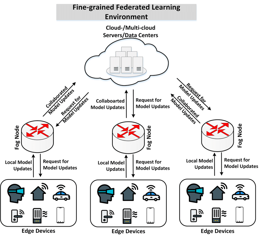
There will be many participants involved in the training process , Each participant has their own data , And train locally , Model parameters will be uploaded after local training , Aggregation of models by a central node pair , Then it is distributed to each participant to synchronize the model .
The advantage of federal learning is , Each node's data is kept local , Ensure data privacy , The access of heterogeneous data is realized ( That is, each participant solves the problem of data access by himself , Even if the data is heterogeneous, it doesn't affect the whole ).
however , Participants still have to upload the model , Will this lead to data privacy leakage ?
Gradient based data restoration
First , Let's formalize the goal first :
x ∗ = arg min x ^ L g r a d ( x ^ ; W , Δ W ) + R a u x ( x ^ ) x^* = \arg \min_{\hat{x}} \mathcal{L}_{grad}(\hat{x};W, \Delta W) + \mathcal{R}_{aux}(\hat{x}) x∗=argx^minLgrad(x^;W,ΔW)+Raux(x^)
among x ^ ∈ R K × C × H × W \hat{x} \in \mathbb{R}^{K\times C\times H\times W} x^∈RK×C×H×W ( K K K yes batch size, C , H , W C,H,W C,H,W The number of channels 、 Height 、 Width ), In the formula W W W It's the weight of the model , Δ W \Delta W ΔW It's the weight change of the aggregated model .
among L g r a d \mathcal{L}_{grad} Lgrad Is the purpose of , Find some possible inputs , So that the weight of training with these inputs , As much as possible consistent with the aggregated weights .
The specific form is
L g r a d ( x ^ ; W , Δ W ) = α G Σ l ∣ ∣ ∇ W ( l ) L ( x ^ , y ^ ) − Δ W ( l ) ∣ ∣ 2 \mathcal{L}_{grad}(\hat{x};W,\Delta W)=\alpha_G\Sigma_{l}||\nabla_{W^{(l)}}\mathcal{L}(\hat{x},\hat{y}) - \Delta W^{(l)}||_2 Lgrad(x^;W,ΔW)=αGΣl∣∣∇W(l)L(x^,y^)−ΔW(l)∣∣2
among Δ W ( l ) = ∇ W ( l ) L ( x ∗ , y ∗ ) \Delta W^{(l)} = \nabla_{W^{(l)}}\mathcal{L}(x^*,y^*) ΔW(l)=∇W(l)L(x∗,y∗), Represent the real training data lead to the second l l l The change of layer weight
There is another term in the previous optimization formula , It's called auxiliary regular term (auxiliary regularization), The specific form is
R a u x ( x ) = R f i d e l i t y ( x ) + R g r o u p ( x ) \mathcal{R}_{aux}(x) = \mathcal{R}_{fidelity}(x) + \mathcal{R}_{group}(x) Raux(x)=Rfidelity(x)+Rgroup(x)
It's made up of two , The first drive x x x Similar to real training samples , The second is consistency , We'll explain later .
Batch label recovery (Batch Label Restoration)
Consider categorizing tasks , Remember that the real data is x ∗ = [ x 1 , x 2 , . . . , x K ] x^* = [x_1,x_2,...,x_K] x∗=[x1,x2,...,xK] , The corresponding label is y ∗ = [ y 1 , y 2 , . . . , y K ] y^* = [y_1,y_2,...,y_K] y∗=[y1,y2,...,yK]
The corresponding real gradient is
∇ W L ( x ∗ , y ∗ ) = 1 K ∑ k ∇ W L ( x k , y k ) \nabla_W\mathcal{L}(x^*,y^*) = \frac{1}{K}\sum_{k}\nabla_W\mathcal{L}(x_k,y_k) ∇WL(x∗,y∗)=K1k∑∇WL(xk,yk)
The error function can be understood as cross entropy (Cross-Entropy) error
In the classification task , The last layer of a network is usually a fully connected linear layer , We record it as W ( F C ) ∈ R M × N W^{(FC)}\in \mathbb{R}^{M\times N} W(FC)∈RM×N
among M M M Is the dimension of the input feature , N N N Is the total number of target categories
For training samples ( x k , y k ) (x_k,y_k) (xk,yk) for , Note that the increment of the linear layer is Δ W m , n , k ( F C ) = ∇ w m , n L ( x k , y k ) \Delta W^{(FC)}_{m,n,k}=\nabla_{w_{m,n}}\mathcal{L}(x_k,y_k) ΔWm,n,k(FC)=∇wm,nL(xk,yk)
Apply the chain rule , You can get :
Δ W m , n , k ( F C ) = ∇ z n , k L ( x k , y k ) × ∂ z n , k ∂ w m , n \Delta W^{(FC)}_{m,n,k} = \nabla_{z_{n,k}}\mathcal{L}(x_k,y_k)\times\frac{\partial z_{n,k}}{\partial w_{m,n}} ΔWm,n,k(FC)=∇zn,kL(xk,yk)×∂wm,n∂zn,k
among z n , k z_{n,k} zn,k Represents the input as x k x_k xk The final process of softmax Layer of the first n n n Outputs , The form of the gradient is
∇ z n , k L ( x k , y k ) = p k , n − y k , n \nabla_{z_{n,k}}\mathcal{L}(x_k,y_k)=p_{k,n} - y_{k,n} ∇zn,kL(xk,yk)=pk,n−yk,n
That is, the probability of the corresponding category minus the tag value
be aware :
∂ z n , k ∂ w m , n = o m , k \frac{\partial z_{n,k}}{\partial w_{m,n}} = o_{m,k} ∂wm,n∂zn,k=om,k
among o m , k o_{m,k} om,k It's the second part of the whole link layer m m m Inputs .
There's a little bit of explanation here , because W ( F C ) ∈ R M × N W^{(FC)}\in \mathbb{R}^{M\times N} W(FC)∈RM×N , The input is a M M M Dimension vector v ∈ R M v \in \mathbb{R}^M v∈RM
For a particular category n n n , The output of z n = v ⋅ W [ : , n ] = ∑ i = 1 M v i w i , n z_n = v\cdot W[:,n] = \sum_{i=1}^{M} v_{i}w_{i,n} zn=v⋅W[:,n]=∑i=1Mviwi,n
that , Immediately ∂ z n , k ∂ w m , n = ∂ ∑ i = 1 M v i w i , n ∂ w m , n = v m \frac{\partial z_{n,k}}{\partial w_{m,n}} = \frac{\partial \sum_{i=1}^{M} v_{i}w_{i,n}}{\partial w_{m,n}} = v_{m} ∂wm,n∂zn,k=∂wm,n∂∑i=1Mviwi,n=vm
v m v_m vm That is to say o m , k o_{m,k} om,k
Because of the input of the linear layer , It's usually through ReLU perhaps sigmoid Activation , So it's generally non negative ,
that , The increment of the parameters of the previous full connection layer Δ W m , n , k ( F C ) = ∇ z n , k L ( x k , y k ) × ∂ z n , k ∂ w m , n \Delta W^{(FC)}_{m,n,k} = \nabla_{z_{n,k}}\mathcal{L}(x_k,y_k)\times\frac{\partial z_{n,k}}{\partial w_{m,n}} ΔWm,n,k(FC)=∇zn,kL(xk,yk)×∂wm,n∂zn,k , Among them ∇ z n , k L ( x k , y k ) \nabla_{z_{n,k}}\mathcal{L}(x_k,y_k) ∇zn,kL(xk,yk) This part , If and only if n = n k ∗ n = n_k^* n=nk∗ ( That is, corresponding to the correct category ) This part is negative .
therefore , For input x k x_k xk , We can identify the target category by the sign of the change amount mentioned above , remember
S n , k = ∑ m Δ W m , n , k ( F C ) = ∑ m ∇ z n , k L ( x k , y k ) × o m , k S_{n,k} = \sum_{m}\Delta W^{(FC)}_{m,n,k}=\sum_{m}\nabla_{z_{n,k}}\mathcal{L}(x_k,y_k)\times o_{m,k} Sn,k=m∑ΔWm,n,k(FC)=m∑∇zn,kL(xk,yk)×om,k
once S n , k < 0 S_{n,k} \lt 0 Sn,k<0 , It means x k x_k xk The category of is n n n
however , All of this is based on a single input x k x_k xk Of , in the light of K K K Inputs , We have
s n = 1 K ∑ k S n , k = ∑ m ( 1 K ∑ k Δ W m , n , k ( F C ) ) s_n = \frac{1}{K}\sum_{k}S_{n,k} = \sum_{m}(\frac{1}{K}\sum_k\Delta W^{(FC)}_{m,n,k}) sn=K1k∑Sn,k=m∑(K1k∑ΔWm,n,k(FC))
This creates a problem : The increment after averaging , There's a loss of information , How to infer categories ?
There is a discovery in this work , namely
∣ S n k ∗ , k ∣ ≫ ∣ S n ≠ n k ∗ , k ∣ |S_{n_k^*, k}| \gg |S_{n\neq n^*_k, k}| ∣Snk∗,k∣≫∣Sn=nk∗,k∣
It means , The significance of the label is still relatively high , We can still infer from its absolute value , also , After gradient aggregation of multiple samples , The negative part is still negative , Showing the information of the original tag .
To make the minus sign more robust , The article uses a column by column minimum , Instead of summing according to characteristic dimensions
namely
y ^ = arg sort ( min m ∇ W m , n ( F C ) L ( x ∗ , y ∗ ) ) [ : K ] \hat{y} = \arg \text{sort}(\min_{m}\nabla_{W^{(FC)}_{m,n}}\mathcal{L}(x^*,y^*))[:K] y^=argsort(mmin∇Wm,n(FC)L(x∗,y∗))[:K]
Let's explain the above formula , First notice ∇ W m , n ( F C ) L ( x ∗ , y ∗ ) ∈ R M × N \nabla_{W^{(FC)}_{m,n}}\mathcal{L}(x^*,y^*) \in \mathbb{R}^{M\times N} ∇Wm,n(FC)L(x∗,y∗)∈RM×N It's a M × N M\times N M×N Matrix
min ∇ W m , n ( F C ) L ( x ∗ , y ∗ ) \min \nabla_{W^{(FC)}_{m,n}}\mathcal{L}(x^*,y^*) min∇Wm,n(FC)L(x∗,y∗) That is to find the smallest line of the matrix , have N N N dimension , And then sort it from small to large ( The negative ones are all ahead )
arg sort \arg \text{sort} argsort In fact, it returns the subscript after sorting , This corresponds to the category , Before going straight back K K K Small value , Which corresponds to K K K Categories of samples
Here's a hypothesis , That is, there is no duplicate category data in a batch , You need to pay attention to !
Authenticity regularization (Fidelity/Realism Regularization)
Here is a reference DeepInversion In view of the picture natural optimization
Dreaming to distill: Data-free knowledge transfer via DeepInversion.
In this paper, a regularization term is added R f i d e l i t y ( ⋅ ) \mathcal{R}_{fidelity}(\cdot) Rfidelity(⋅), To drive generation x ^ \hat{x} x^ Keep it as real as possible , The specific form is :
R f i d e l i t y ( x ^ ) = α t v R T V ( x ^ ) + α l 2 R l 2 ( x ^ ) + α B N R B N ( x ^ ) \mathcal{R}_{fidelity}(\hat{x}) = \alpha_{tv}\mathcal{R}_{TV}(\hat{x}) + \alpha_{l_2}\mathcal{R}_{l_2}(\hat{x}) + \alpha_{BN}\mathcal{R}_{BN}(\hat{x}) Rfidelity(x^)=αtvRTV(x^)+αl2Rl2(x^)+αBNRBN(x^)
among R T V \mathcal{R}_{TV} RTV and R l 2 \mathcal{R}_{l_2} Rl2 Penalize the variance of the image and L 2 L2 L2 norm , Belongs to the standard image prior .
DeepInversion The key part of this is the use of BN To constrain... A priori
R B N ( x ^ ) = ∑ l ∣ ∣ μ l ( x ^ ) − B N l ( m e a n ) ∣ ∣ 2 + ∑ l ∣ ∣ σ l 2 ( x ^ ) − B N l ( v a r i a n c e ) ∣ ∣ 2 \mathcal{R}_{BN}(\hat{x}) = \sum_{l}||\mu_l(\hat{x}) - BN_l(mean)||_2 +\sum_{l}||\sigma_l^2(\hat{x}) - BN_l(variance)||_2 RBN(x^)=l∑∣∣μl(x^)−BNl(mean)∣∣2+l∑∣∣σl2(x^)−BNl(variance)∣∣2
among μ l ( x ) \mu_l(x) μl(x) and σ l 2 ( x ) \sigma_l^2(x) σl2(x) It's No l l l Layer convolution , Estimation of the mean and variance of a batch of data
This regularization of authenticity can make the image more realistic
Group consistent regularization (Group Consistency Regularization)
In the process of training data recovery , There will be a challenge , That is, the determination of the actual position of the object , As shown in the figure below :

In the experiment , The author uses different random seeds to restore the image , The result is different degrees of offset , But these samples are semantically consistent .
Based on this observation , A regularization method for group consistency is proposed , That is to say, different random seeds are used to generate , And then fuse these results .
The regularized form is :
R g r o u p ( x ^ , x ^ g ∈ G ) = α g r o u p ∣ ∣ x ^ − E ( x ^ g ∈ G ) ∣ ∣ 2 \mathcal{R}_{group}(\hat{x},\hat{x}_{g\in G}) = \alpha_{group}||\hat{x}-\mathbb{E}(\hat{x}_{g\in G})||_2 Rgroup(x^,x^g∈G)=αgroup∣∣x^−E(x^g∈G)∣∣2
among , We need to work out this expectation E ( x ^ g ∈ G ) \mathbb{E}(\hat{x}_{g\in G}) E(x^g∈G), In fact, that is Average image 
As shown in the figure above , First, average by pixels , Get an average image , Then all the images are aligned based on this average image , Then take the average again , Get the final aligned average image .
Final update details
An energy based model is used in this paper , suffer Langevin Inspired by the , The specific form is
Δ x ^ ( t ) ← ∇ x ^ ( L g r a d ( x ^ ( t − 1 ) , ∇ W ) + R a u x ( x ^ ( t − 1 ) ) ) η ← N ( 0 , I ) x ^ ( t ) ← x ^ ( t − 1 ) + λ ( t ) Δ x ^ ( t ) + λ ( t ) α n η \Delta_{\hat{x}^{(t)}} \leftarrow \nabla_{\hat{x}}(\mathcal{L}_{grad}(\hat{x}^{(t-1)},\nabla W) + \mathcal{R}_{aux}(\hat{x}^{(t-1)}))\\ \eta \leftarrow \mathcal{N}(0, I)\\ \hat{x}^{(t)} \leftarrow \hat{x}^{(t-1)} + \lambda(t)\Delta_{\hat{x}^{(t)}} + \lambda(t)\alpha_n\eta Δx^(t)←∇x^(Lgrad(x^(t−1),∇W)+Raux(x^(t−1)))η←N(0,I)x^(t)←x^(t−1)+λ(t)Δx^(t)+λ(t)αnη
among η \eta η It's sampling noise , For searching ; λ ( t ) \lambda(t) λ(t) It's the learning rate ; α n \alpha_n αn It's the zoom factor .
experimental analysis
First of all, let's look at the correct rate of label recovery
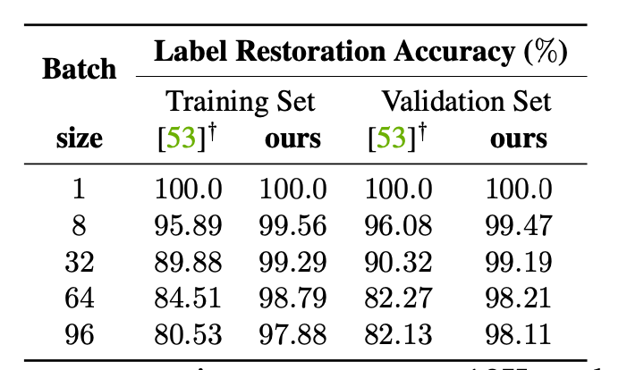
You can see , As the batch size increases , The accuracy will drop , The reason is actually the problem of repeating categories , But compared to iDLG Is much better .
iDLG: Improved deep leakage from gradients.
Then there is the Ablation Experiment of each error term

You can see , Add authenticity and group consistency , It does improve the quality of the picture , The gain of alignment also exists .
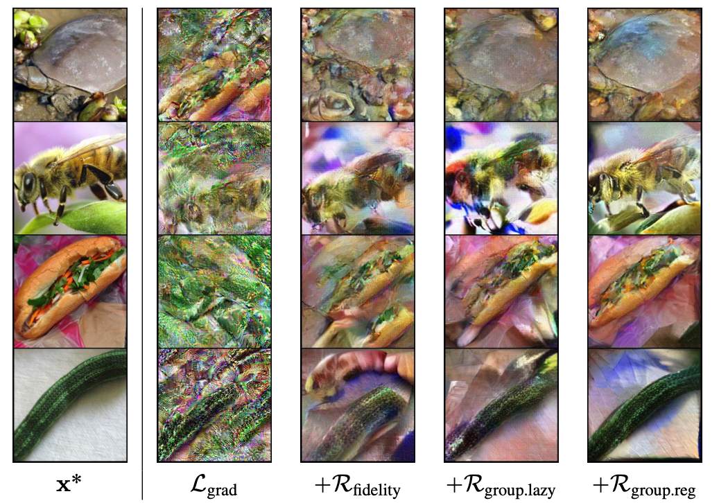
As shown in the figure above , Basically, the result of restoration is close to the original image
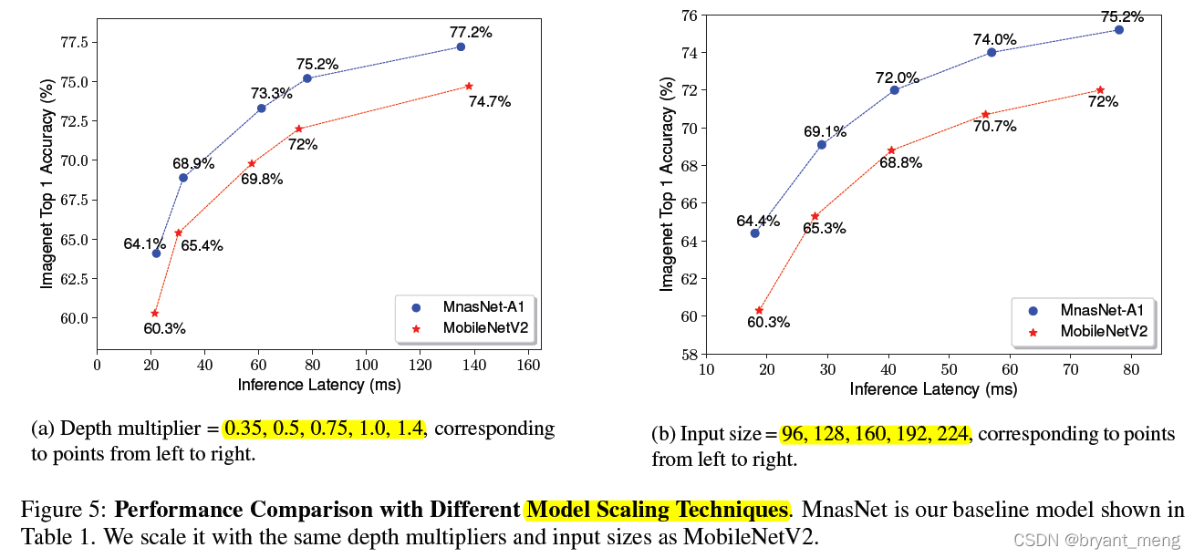
then , And current SOTA Compare the effect , Here is a part of the result graph

You can see , The effect is better than DeepInversion,Latent Projection It's much better to wait for work !
after , We have to look at the batch size , That is to say BatchSize, The effect on the reduction effect
[ Failed to transfer the external chain picture , The origin station may have anti-theft chain mechanism , It is suggested to save the pictures and upload them directly (img-LlXEZOc0-1620807309508)(…/…/…/…/…/Application Support/typora-user-images/image-20210512160851739.png)]
You can see , As the batch size increases , The reduction effect will be worse , It's also common sense , Because the information loss caused by aggregation will increase .
Conclusion
This work is a milestone , In the context of federal learning , Achieved a powerful attack !
It's going to be a great inspiration , For the follow-up defense work under the scenario of distributed training such as federated learning .
DP And so on ? Whether changes in participants will have an impact ? Does the local training increase the difficulty of recovery ?
There is still a lot of work we need to explore together .
边栏推荐
- Several methods of image enhancement and matlab code
- 【Sparse-to-Dense】《Sparse-to-Dense:Depth Prediction from Sparse Depth Samples and a Single Image》
- Summary of open3d environment errors
- 【双目视觉】双目矫正
- 【Hide-and-Seek】《Hide-and-Seek: A Data Augmentation Technique for Weakly-Supervised Localization xxx》
- (15) Flick custom source
- open3d学习笔记二【文件读写】
- EKLAVYA -- 利用神经网络推断二进制文件中函数的参数
- Common machine learning related evaluation indicators
- How gensim freezes some word vectors for incremental training
猜你喜欢
【MnasNet】《MnasNet:Platform-Aware Neural Architecture Search for Mobile》

Timeout docking video generation

【雙目視覺】雙目矯正

It's great to save 10000 pictures of girls
Correction binoculaire

Programmers can only be 35? The 74 year old programmer in the United States has been programming for 57 years and has not retired
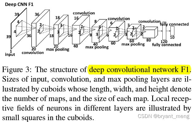
【Cascade FPD】《Deep Convolutional Network Cascade for Facial Point Detection》

用MLP代替掉Self-Attention
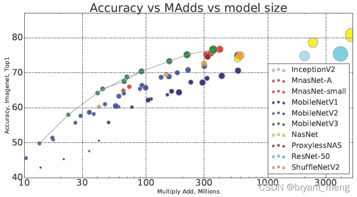
【MobileNet V3】《Searching for MobileNetV3》
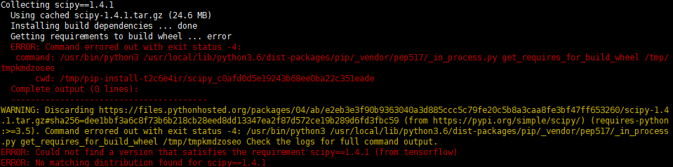
jetson nano安装tensorflow踩坑记录(scipy1.4.1)
随机推荐
【学习笔记】Matlab自编图像卷积函数
Correction binoculaire
【FastDepth】《FastDepth:Fast Monocular Depth Estimation on Embedded Systems》
【Batch】learning notes
Rhel7 operation level introduction and switching operation
C语言的库函数
Business architecture diagram
Open3D学习笔记一【初窥门径,文件读取】
AR系统总结收获
C # connect to MySQL database
E-R draw clear content
Embedding malware into neural networks
What if a new window always pops up when opening a folder on a laptop
【DIoU】《Distance-IoU Loss:Faster and Better Learning for Bounding Box Regression》
【Cutout】《Improved Regularization of Convolutional Neural Networks with Cutout》
【Programming】
【Mixed Pooling】《Mixed Pooling for Convolutional Neural Networks》
Proof and understanding of pointnet principle
针对语义分割的真实世界的对抗样本攻击
Solve the problem of latex picture floating