当前位置:网站首页>Chapter 5 neural network
Chapter 5 neural network
2022-07-08 01:07:00 【Intelligent control and optimization decision Laboratory of Cen】
1. Try to describe common activation functions , Try to describe the linear function f ( x ) = w T x f(x)=w^Tx f(x)=wTx Defects used as neuron activation function
1.1 What is an activation function
Here's the picture , Here's the picture , In neurons , Input inputs By weighting , After summing up , A function is also applied , This function is the activation function Activation Function.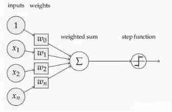
1.2 The function of activation
If you don't use the excitation function , The output of each layer is a linear function of the upper input , No matter how many layers the neural network has , The output is a linear combination of inputs , This is why linear activation functions are not used .
If used , Activation functions introduce nonlinear factors into neurons , So that the neural network can arbitrarily approximate any nonlinear function , So the neural network can be applied to many nonlinear models .
1.3 Common activation functions
- Sigmoid Activation function
sigmoid Is the most widely used type of activation function , With exponential function shape , It is closest to biological neuron in physical sense . Besides , ( 0 , 1 ) (0, 1) (0,1) The output of can also be expressed as probability , Or normalization for input , Typical examples are Sigmoid Cross entropy loss function .
However ,sigmoid It also has its own shortcomings , The most obvious is saturation . You can see it in the picture below , Its derivatives on both sides gradually approach 0 . Those with this property are called soft saturation activation functions . Concrete , Saturation can be divided into left saturation and right saturation . Corresponding to soft saturation is hard saturation .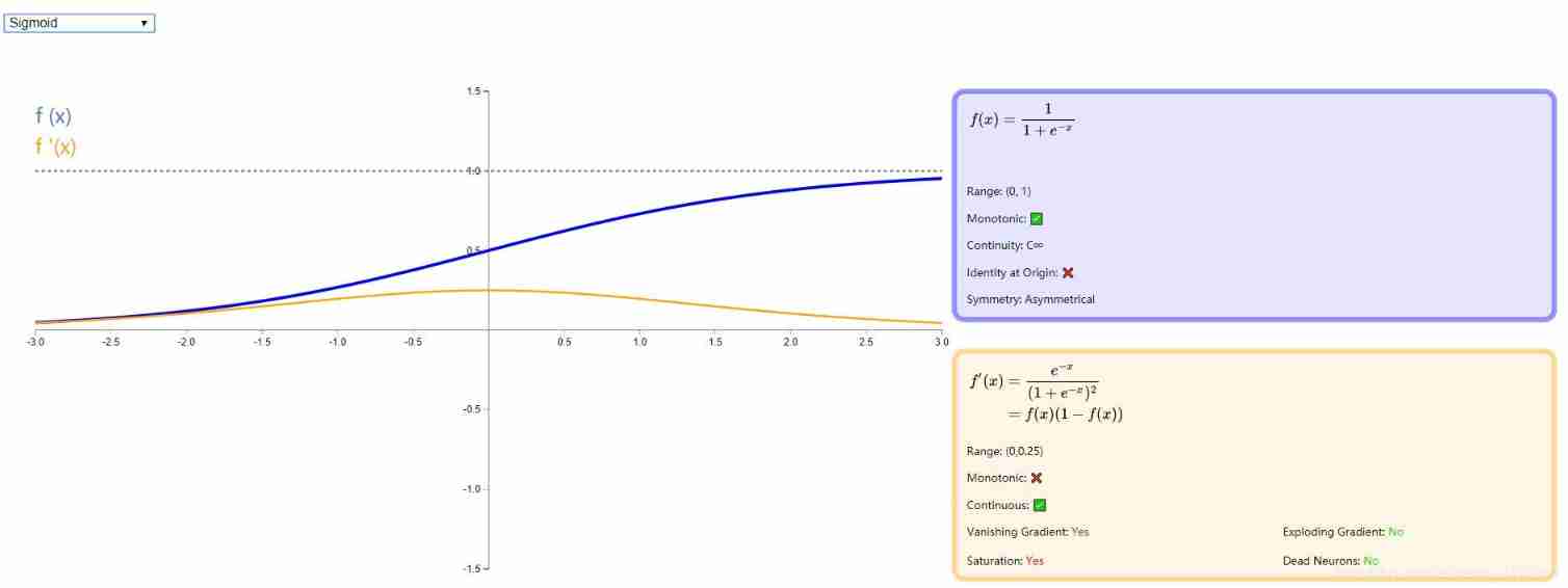
- Tanh function
tanh Is a hyperbolic tangent function ,tanh Functions and sigmod The curve of the function is relatively similar , Let's compare . First of all, the same is , When the input of these two functions is large or small , The output is almost smooth , The gradient is very small , It is not conducive to weight update ; The difference is the output interval ,tanh The output interval of is in (-1,1) Between , And the whole function is based on 0 Centred , This feature is better than sigmod Good. .
In general binary classification problems , Hidden layer with tanh function , For output layer sigmod function . But these are not invariable , What activation function is used , Or we should analyze it according to specific problems , It still depends on debugging .
See the figure below for details :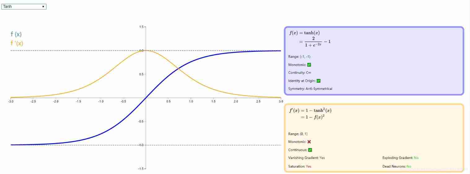
- ReLU
ReLU The full name is :Rectified linear unit, It is a popular activation function at present , It retains something similar step That biological neuronal mechanism : When the input exceeds the threshold, it will fire . Although in 0 Points cannot be derived , However, it does not affect its effective role in gradient based back propagation . of ReLU Detailed introduction , Please move on to the paper :《Rectified Linear Units Improve Restricted Boltzmann Machines》 There is also a blog with a comprehensive introduction : Neural network review - Relu Activation function .
Here is the following :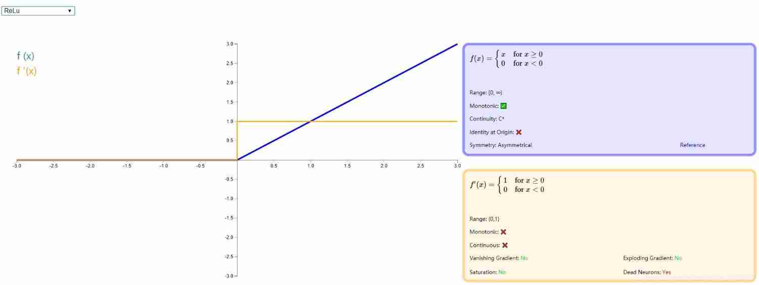
- Leaky ReLU
because ReLU All parts less than zero are classified as 0 , This is very easy to cause Neuron death , therefore Andrew L. Maas Wait for someone in the paper 《Rectifier Nonlinearities Improve Neural Network Acoustic Models》 A new activation function is proposed in , In less than 0 Add a very small slope in the direction of . Here's the picture :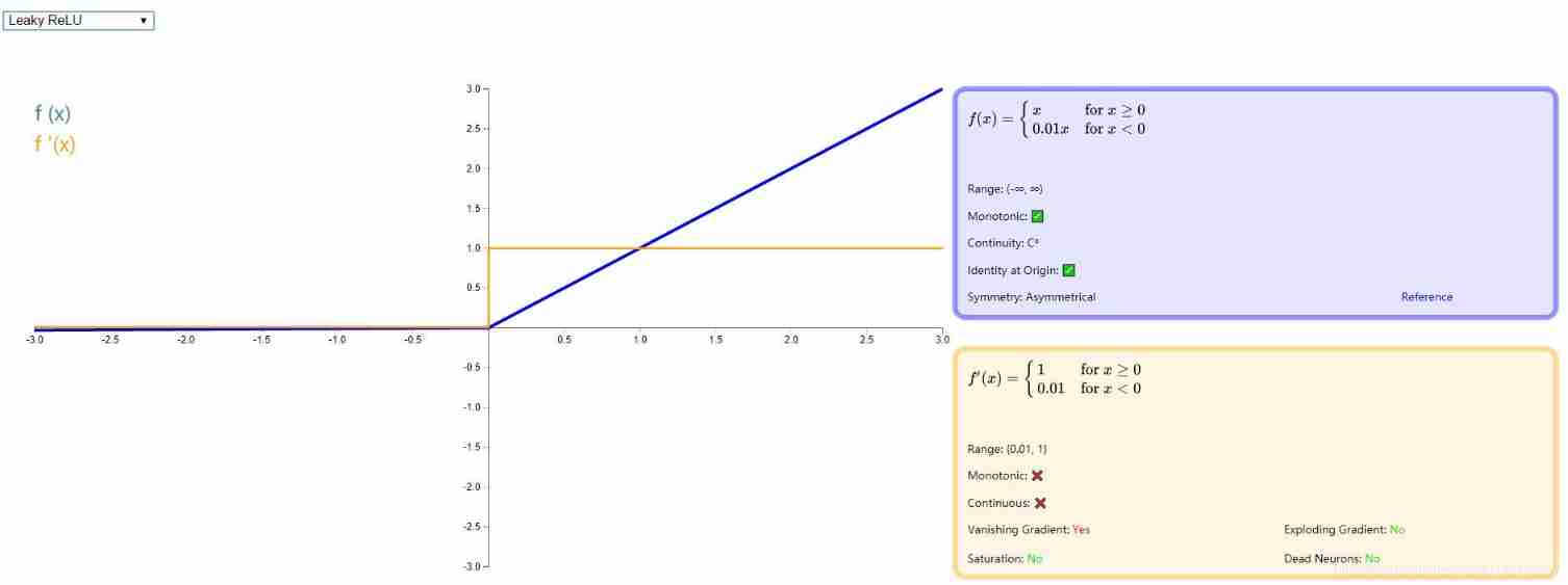
2. Perceptrons and multilayer networks
2.1 perceptron
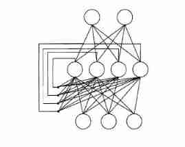
perceptron (Perceptron) It's made up of two layers of neurons , As shown in the figure , The input layer receives the external input signal and passes it to the output layer , The output layer is M−PM−P Neuron , Also known as “ Threshold logical unit ”.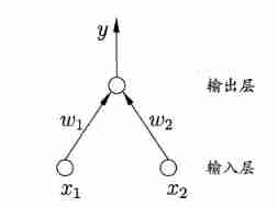
More generally , Given the training data set , The weight w i w_i wi And the threshold θ \theta θ You can learn . threshold θ \theta θ It can be regarded as a fixed input − 1.0 -1.0 −1.0 Of “ Dumb node ” Multiple corresponding connection weights w n + 1 w_{n+1} wn+1. such , Weight and threshold learning can be unified as weight learning . The learning rules of perceptron are very simple , For training samples ( x , y ) (x,y) (x,y), If the output of the current sensor is y ^ \hat y y^, Then the weight of the perceptron will be optimally adjusted :
w i ← w i + Δ w i Δ w i = η ( y − y ^ ) x i w_i \leftarrow w_i +\Delta w_i \\ \Delta w_i=\eta(y-\hat y)x_i wi←wi+ΔwiΔwi=η(y−y^)xi
among η ∈ ( 0 , 1 ) \eta \in (0,1) η∈(0,1) be called “ Learning rate (learing rate)” . It can be seen from the above formula , If the perceptron is on the training sample ( x , y ) (x,y) (x,y) The prediction is correct , Then the perceptron does not change , Otherwise, the weight will be adjusted according to the degree of error . The perceptron has only output layer neurons to process the activation function , That is, only one layer of functional neurons , Their learning ability is very limited . It can only deal with linearly separable cases , Unable to deal with non-linear separable cases .
2.2 Multi layer network
To solve the nonlinear separable problem , We need to consider using multi-layer functional neurons . A layer of neurons between the output layer and the input layer , It is called hidden layer or hidden layer , Hidden layer and output layer neurons are functional neurons with activation function .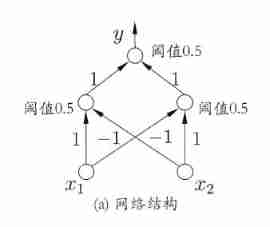
More generally , Common neural networks are shown in the figure below , Each layer of neurons is fully interconnected with the next layer of neurons , There is no same layer connection between neurons , There is no cross layer connection . Such neural network results are usually called “ Multilayer feedforward neural network ”(multi-layer feedforward neural networks), The input layer neuron receives external input , Hidden layer and output layer neurons process signals , The final result is output by the output layer neurons ; In other words , Input layer neurons only accept input , No function processing , The hidden layer and the output layer contain functional neurons .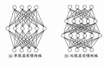
3. Try to use sigmoid The relationship between neurons of activation function and logarithmic probability regression .
Both are related to s i g m o i d sigmoid sigmoid Function related , But in logarithmic probability regression , s i g m o i d sigmoid sigmoid The function is to convert the predicted value generated by the linear regression model ( It's worth it ) Turn into 0 / 1 0/1 0/1 value . s i g m o i d sigmoid sigmoid Function is used to replace unit step function , because s i g m o i d sigmoid sigmoid The function is monotonic and differentiable ; In the neuron model , s i g m o i d sigmoid sigmoid Function as “ Activation function ” Used to process the output of neurons , Because neurons in the neuron model receive signals from n n n The input signals from these other neurons , These input signals are transmitted through weighted connections , The total input received by the neuron is compared with the threshold of the neuron , use “ Activation function ” It can convert the output value into 0 / 1 0/1 0/1 value .
3. For Graphs 5.7(102 page ) Medium , Try to deduce BP Update formula in the algorithm
For training example ( x k , y k ) (\bm x_k,\bm y_k) (xk,yk), Suppose the output of the neural network is y ^ k = ( y ^ 1 k , y ^ 2 k , . . . , y ^ l k ) \hat y_k=(\hat y_{1}^{k},\hat y_{2}^{k},...,\hat y_{l}^{k}) y^k=(y^1k,y^2k,...,y^lk), namely y ^ j k = f ( β j − θ j ) \hat y_{j}^{k}=f(\beta_j-\theta_j) y^jk=f(βj−θj) ,
Then the network is ( x k , y k ) (\bm x_k,\bm y_k) (xk,yk) The mean square error of is :
E k = 1 2 ∑ j = 1 l ( y ^ j k − y ^ j k ) 2 E_k=\frac{1}{2}\sum_{j=1}^{l}(\hat y_{j}^{k}-\hat y_{j}^{k})^2 Ek=21j=1∑l(y^jk−y^jk)2
Arbitrary parameters v v v The updated estimation formula is v ← v + Δ v v \leftarrow v+ \Delta v v←v+Δv
For errors E k E_k Ek, Given the learning rate η \eta η, Yes Δ w h j = − η ∂ E k ∂ w h j . \Delta w_{hj}=-\eta \frac{\partial E_k}{\partial w_{hj}}. Δwhj=−η∂whj∂Ek.
Can be derived :
∂ E k ∂ w h j = ∂ E k ∂ y ^ j k . ∂ y ^ j k ∂ β j . ∂ β j ∂ w h j . ∂ β j ∂ w h j = b h f ′ ( x ) = f ( x ) ( 1 − f ( x ) ) g j = − ∂ E k ∂ y ^ j k . ∂ y ^ j k ∂ β j = − ( y ^ j k − y j k ) f ′ ( β j − θ j ) = y ^ j k ( 1 − y ^ j k ) ( y j k − y ^ j k ) \frac{\partial E_k} {\partial w_{hj}}=\frac{\partial E_k} {\partial \hat y_{j}^{k}}.\frac{\partial \hat y_{j}^{k}} {\partial \beta _j}.\frac{\partial \beta _j} {\partial w_{hj}} . \\ \ \ \frac{\partial \beta _j} {\partial w_{hj}}=b_h \\ f'(x)=f(x)(1-f(x)) \\ g_j= -\frac{\partial E_k} {\partial \hat y_{j}^{k}}.\frac{\partial \hat y_{j}^{k}} {\partial \beta _j} \\ \ \ \ \ \ \ \ \ \ \ \ \ \ \ \ \ \ \ \ \ \ \ =-(\hat y_{j}^{k}-y_{j}^{k})f'(\beta_j-\theta _j)\\ \ \ \ \ \ \ \ \ \ \ \ \ \ \ \ \ \ =\hat y_{j}^{k}(1-\hat y_{j}^{k})(y_{j}^{k}-\hat y_{j}^{k}) ∂whj∂Ek=∂y^jk∂Ek.∂βj∂y^jk.∂whj∂βj. ∂whj∂βj=bhf′(x)=f(x)(1−f(x))gj=−∂y^jk∂Ek.∂βj∂y^jk =−(y^jk−yjk)f′(βj−θj) =y^jk(1−y^jk)(yjk−y^jk)
And then you get it BP The algorithm is about w h j w_{hj} whj The updated formula of Δ w h j = η g j b h . \Delta w_{hj}=\eta {g_j}{b_h.} Δwhj=ηgjbh.
Similar can be obtained Δ θ j = − η g j , Δ v i h = η e h x i , Δ γ = − η e h , \Delta \theta_j=-\eta g_j ,\\ \Delta v_{ih}=\eta e_h x_i,\\ \Delta \gamma=-\eta e_h, Δθj=−ηgj,Δvih=ηehxi,Δγ=−ηeh,
among e h = ∂ E k ∂ b h . ∂ b h ∂ α h = − ∑ j = 1 l ∂ E k ∂ β j . ∂ β j ∂ b h f ′ ( α h − γ h ) = ∑ j = 1 l w h j g j f ′ ( α h − γ h ) = b h ( 1 − b h ) ∑ j = 1 l w h j g j e_h=\frac{\partial E_k}{\partial b_h}.\frac{\partial b_h}{\partial \alpha_h } \\ =-\sum_{j=1}^{l}\frac{\partial E_k}{\partial \beta_j}.\frac{\partial \beta_j}{\partial b_h}f'(\alpha_h-\gamma_h) \\ =\sum_{j=1}^{l}w_{hj}g_jf'(\alpha_h-\gamma_h)\\ =b_h(1-b_h)\sum_{j=1}^{l}w_{hj}g_j eh=∂bh∂Ek.∂αh∂bh=−j=1∑l∂βj∂Ek.∂bh∂βjf′(αh−γh)=j=1∑lwhjgjf′(αh−γh)=bh(1−bh)j=1∑lwhjgj
4. Try to describe the standard BP Algorithm and accumulation BP Algorithm , Try programming to realize the standard BP Algorithm and accumulation BP Algorithm , Using these two algorithms to train a single hidden layer neural network on watermelon data set , And compare
Here's the thing , BP The goal of the algorithm is to minimize the training set D D D Cumulative error on
E = 1 m ∑ k = 1 m E k E=\frac{1}{m}\sum_{k=1}^{m}E_k E=m1k=1∑mEk But what we introduced above " standard BP Algorithm " Update the connection weights and thresholds for only one training sample at a time , in other words , The update rules of the algorithm are based on a single E k E_k Ek Derived from . As a result, an update rule based on the minimization of cumulative error is similarly derived , The cumulative error inverse propagation is obtained (accumulated error backpropagation) Algorithm . The cumulative BP Algorithms and standards BP Algorithms are commonly used . Generally speaking , standard BP Each update of the algorithm is only for a single sample , Parameters are updated very frequently , Moreover, the effect of updating different samples may appear " offset " The phenomenon . therefore , In order to achieve the same cumulative error minimum , standard BP Algorithms often need more iterations . The cumulative BP The algorithm directly aims at minimizing the cumulative error , It's reading the entire training set D D D Update parameters after one pass , The frequency of parameter update is much lower . But in many tasks , After the cumulative error decreases to a certain extent , Further decline will be very slow , Standard at this time BP Better solutions tend to be obtained faster , Especially in the training set D D D It is more obvious when it is very large .
5. Try to describe how to alleviate BP Over fitting phenomenon of neural network
because BP(BackPropagation) Neural network has strong representation ability ,PB Neural networks often encounter fitting , The training error continues to decrease , But test errors can go up . There are two strategies commonly used to alleviate BP Overfitting of networks :
- The first strategy is “ Stop early ”(early stopping): Divide the data into training set and verification set , The training set is used to calculate the gradient 、 Update connection rights and thresholds , The verification set is used to estimate the error , If the training set error decreases but the verification set error increases , Then stop training , At the same time, the connection weight and threshold with the minimum verification set error are returned .
- The second strategy is “ Regularization ”(regularization), The basic idea is to add a part to the error objective function to describe the network complexity , For example, the sum of the squares of the connection weight and the threshold .
6. Try to explain RBF The Internet ,RNN Concept and characteristics of recurrent neural network
RBF It is a single hidden layer feedforward neural network , It uses the radial basis function as the activation function of hidden layer neurons , The output layer is a linear combination of the outputs of neurons in the hidden layer , Suppose the input is d d d Dimension vector x \bm x x, Output as real value , be RBF Can be expressed as
φ ( x ) = ∑ i = 1 q ρ ( x , c i ) \varphi(\bm x)=\sum_{i=1}^{q}\rho(\bm x,\bm c_i) φ(x)=i=1∑qρ(x,ci)
among q q q Is the number of neurons in the hidden layer , c i and w i c_i and w_i ci and wi They are the first i i i The center and weight of each hidden layer neuron , ρ ( x , c i ) \rho(x,c_i) ρ(x,ci) Is the radial basis function , This is a function of radial symmetry , Usually defined as a sample x x x To the data center c i c_i ci A monotonic function of the Euclidean distance between . Common Gaussian radial basis functions are shaped like :
ρ ( x , c i ) = e − β i ∣ ∣ x − c i ∣ ∣ 2 \rho (x,c_i)=e^{-\beta_i||x-c_i||^2} ρ(x,ci)=e−βi∣∣x−ci∣∣2 With enough hidden neurons RBF Neural network can approximate any continuous function with any accuracy .RNN Cyclic neural network , Different from feedforward neural network ,“ Recursive neural network ”(Recurrent Neural Networks) Allow the network to have a ring structure , The output of some neurons can be fed back as input signals , That is, the network is t t t The output state of the time is not only related to the input , And also t − 1 t-1 t−1 The network state at the moment , Thus, it can deal with the dynamic changes related to time .Elman Network is one of the most commonly used recurrent neural networks , Its structure is similar to multilayer feedforward network , But the output of hidden layer neurons is fed back , Together with the signal provided by the input layer neuron at the next moment , As the input of hidden layer neurons at the next moment . Hidden layer neurons usually adopt S i g m o i d Sigmoid Sigmoid Activation function , And network training is often promoted BP Algorithm .
7. Try to describe the convolution of convolution neural network 、 Down sampling ( Pooling ) The process , Try to describe the architecture of convolutional neural network
From a computer point of view , The image is actually a two-dimensional matrix , The work of convolution neural network is to use convolution 、 Operations such as pooling extract features from two-dimensional arrays , And recognize the image . In theory , As long as it is data that can be converted into a two-dimensional matrix , Convolutional neural network can be used to identify and detect . For example, sound files , It can be divided into very short segments , The height of each scale can be converted into numbers , In this way, the whole sound file can be converted into a two-dimensional matrix , Similar to text data in natural language , Chemical data in medical experiments and so on , Convolutional neural network can be used to realize recognition and detection .
Convolution : Convolution is the core concept of convolutional neural network , It is also the origin of its name . Convolution is used to extract local features of an image , It is a mathematical calculation method , The following figure vividly shows the convolution process .

Pooling
Pool English is pooling, Another name is down sampling( Down sampling ), I have to say that the translation of these two terms is very faithful to the original meaning , But this kind of straightforward translation is very difficult to understand . Use popular language to describe : Pooling is to divide the characteristic matrix into several small blocks , Select a value from each sub matrix to replace the sub matrix , The purpose of this is to compress the characteristic matrix , Simplify the next calculation . There are two ways to pool :Max Pooling( Maximum pooling ) and Average Pooling( Average pooling ), The former is to take the maximum value from the submatrix , The latter is to take the average .
Pooling is easier to understand than convolution , The dynamic diagram above simulates a simple pooling process , The Yellow characteristic matrix is divided into four sub matrices , Then select a value from each sub matrix according to the pooling method to form the pooling matrix . Maximum pooling is a commonly used pooling method , Because selecting the maximum value of the region can well maintain the characteristics of the original image .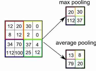
Convolutional neural network architecture
Here is a common convolutional neural network CNN Basic architecture , As shown in the figure , Network input is a 32 × 32 32×32 32×32 The handwritten digital image of , The output is its recognition result ,CNN Compound multiple “ Convolution layer ” and “ Sampling layer ” Process the input signal . Then the mapping between the connection layer and the output target . Each convolution layer contains multiple feature maps , Each feature map is composed of multiple neurons “ Plane ”, A feature of the input is extracted by a convolution filter .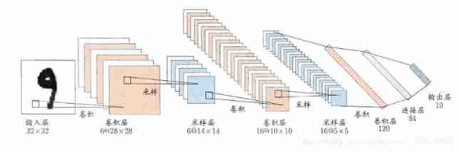
8. kaggle Introduction to the game - Handwritten digit recognition , Download data and code , Read the code carefully and mark the code comments in detail .
Reference data :
https://www.kaggle.com/c/digit-recognizer/overview
Reference code :
https://www.kaggle.com/elcaiseri/mnist-simple-cnn-keras-accuracy-0-99-top-1
边栏推荐
猜你喜欢
3.MNIST数据集分类

Vscode is added to the right-click function menu
How to transfer Netease cloud music /qq music to Apple Music
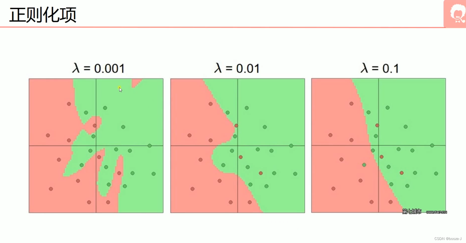
5. Over fitting, dropout, regularization
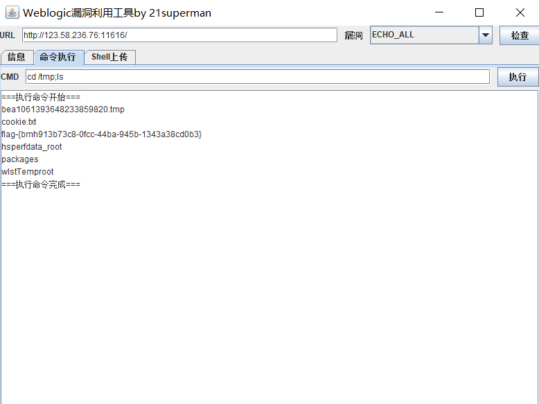
FOFA-攻防挑战记录
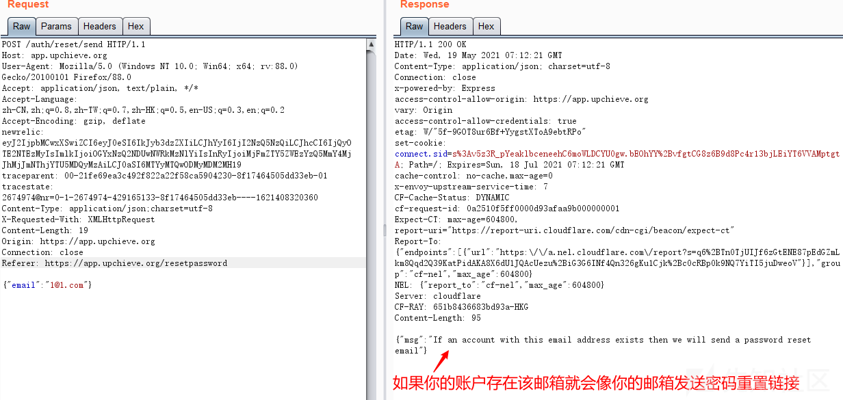
国外众测之密码找回漏洞
Su embedded training - Day9
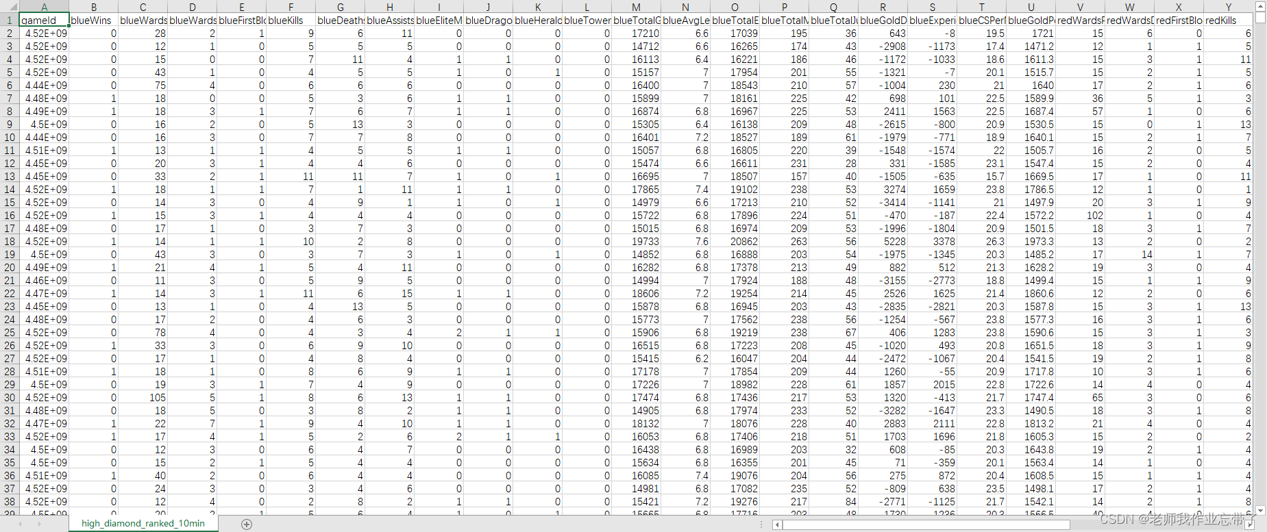
英雄联盟胜负预测--简易肯德基上校

Image data preprocessing

From starfish OS' continued deflationary consumption of SFO, the value of SFO in the long run
随机推荐
2. Nonlinear regression
1.线性回归
10. CNN applied to handwritten digit recognition
Prediction of the victory or defeat of the League of heroes -- simple KFC Colonel
Serial port receives a packet of data
From starfish OS' continued deflationary consumption of SFO, the value of SFO in the long run
A network composed of three convolution layers completes the image classification task of cifar10 data set
STL--String类的常用功能复写
Binder core API
What does interface testing test?
Cross modal semantic association alignment retrieval - image text matching
Service Mesh的基本模式
Image data preprocessing
My best game based on wechat applet development
Mathematical modeling -- knowledge map
jemter分布式
11.递归神经网络RNN
50MHz generation time
10.CNN应用于手写数字识别
Semantic segmentation model base segmentation_ models_ Detailed introduction to pytorch