当前位置:网站首页>Map of mL: Based on the adult census income two classification prediction data set (whether the predicted annual income exceeds 50K), use the map value to realize the interpretable case of xgboost mod
Map of mL: Based on the adult census income two classification prediction data set (whether the predicted annual income exceeds 50K), use the map value to realize the interpretable case of xgboost mod
2022-07-06 06:44:00 【A Virgo procedural ape】
ML And shap: be based on adult Census income two classification forecast data set ( Whether the predicted annual income exceeds 50k) utilize Shap It's worth it XGBoost A detailed introduction to interpretable cases of model implementation
Catalog
# 2.1、 Preliminary screening of modeling features
# 2.2、 Target feature binarization
# 2.3、 Category feature coding digitization
# 2.4、 Separate features from labels
#3、 Model training and reasoning
# 3.2、 Model building and training
#4、 Model feature importance interpretation visualization
#4.1、 Visualization of global feature importance
# T1、 Output the importance of features based on the model itself
# T2、 utilize Shap Value interpretation XGBR Model
#4.2、 Visualization of local feature importance
# (1)、 Single sample full feature bar graph visualization
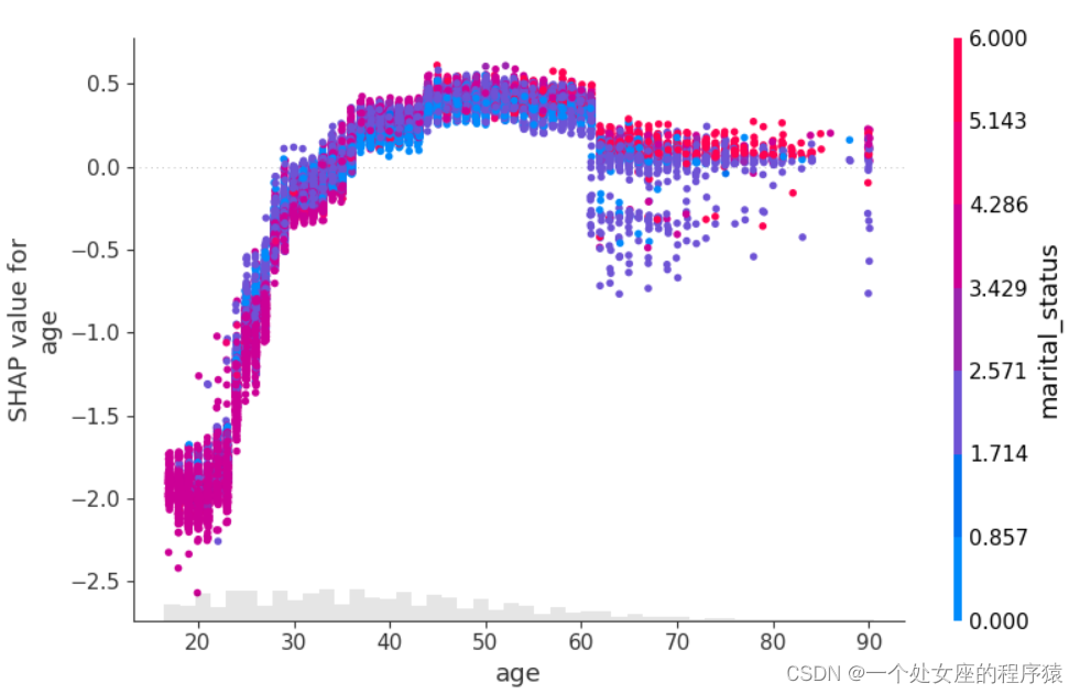
# (2)、 One turn two feature full sample local independent graph scatter diagram visualization
# (3)、 Visualization of double feature full sample scatter diagram
# 4.3、 Model feature screening
# (1)、 Clustering based shap Feature filtering visualization
5、 Interpretability of model prediction ( It can mainly analyze misclassified samples )
(1)、 A single sample tries to visualize — Compare predictions
(2)、 Multiple samples try to visualize
# 5.2、 Visual analysis of decision diagram : How models make decisions
# (1)、 Single sample decision graph visualization
# (2)、 Visualization of multiple sample decision diagrams
be based on adult Census income two classification forecast data set ( Whether the predicted annual income exceeds 50k) utilize Shap It's worth it XGBoost Model implementation interpretability case
1、 Define datasets
dtypes_len: 15
| age | workclass | fnlwgt | education | education_num | marital_status | occupation | relationship | race | sex | capital_gain | capital_loss | hours_per_week | native_country | salary |
| 39 | State-gov | 77516 | Bachelors | 13 | Never-married | Adm-clerical | Not-in-family | White | Male | 2174 | 0 | 40 | United-States | <=50K |
| 50 | Self-emp-not-inc | 83311 | Bachelors | 13 | Married-civ-spouse | Exec-managerial | Husband | White | Male | 0 | 0 | 13 | United-States | <=50K |
| 38 | Private | 215646 | HS-grad | 9 | Divorced | Handlers-cleaners | Not-in-family | White | Male | 0 | 0 | 40 | United-States | <=50K |
| 53 | Private | 234721 | 11th | 7 | Married-civ-spouse | Handlers-cleaners | Husband | Black | Male | 0 | 0 | 40 | United-States | <=50K |
| 28 | Private | 338409 | Bachelors | 13 | Married-civ-spouse | Prof-specialty | Wife | Black | Female | 0 | 0 | 40 | Cuba | <=50K |
| 37 | Private | 284582 | Masters | 14 | Married-civ-spouse | Exec-managerial | Wife | White | Female | 0 | 0 | 40 | United-States | <=50K |
| 49 | Private | 160187 | 9th | 5 | Married-spouse-absent | Other-service | Not-in-family | Black | Female | 0 | 0 | 16 | Jamaica | <=50K |
| 52 | Self-emp-not-inc | 209642 | HS-grad | 9 | Married-civ-spouse | Exec-managerial | Husband | White | Male | 0 | 0 | 45 | United-States | >50K |
| 31 | Private | 45781 | Masters | 14 | Never-married | Prof-specialty | Not-in-family | White | Female | 14084 | 0 | 50 | United-States | >50K |
| 42 | Private | 159449 | Bachelors | 13 | Married-civ-spouse | Exec-managerial | Husband | White | Male | 5178 | 0 | 40 | United-States | >50K |
2、 Data set preprocessing
# 2.1、 Preliminary screening of modeling features
df.columns
14
# 2.2、 Target feature binarization
# 2.3、 Category feature coding digitization
filt_dtypes_len: 13 [('age', 'float32'), ('workclass', 'category'), ('fnlwgt', 'float32'), ('education_Num', 'float32'), ('marital_status', 'category'), ('occupation', 'category'), ('relationship', 'category'), ('race', 'category'), ('sex', 'category'), ('capital_gain', 'float32'), ('capital_loss', 'float32'), ('hours_per_week', 'float32'), ('native_country', 'category')]
# 2.4、 Separate features from labels
df_adult_display
| age | workclass | education_num | marital_status | occupation | relationship | race | sex | capital_gain | capital_loss | hours_per_week | native_country | salary | |
| 0 | 39 | State-gov | 13 | Never-married | Adm-clerical | Not-in-family | White | Male | 2174 | 0 | 40 | United-States | 0 |
| 1 | 50 | Self-emp-not-inc | 13 | Married-civ-spouse | Exec-managerial | Husband | White | Male | 0 | 0 | 13 | United-States | 0 |
| 2 | 38 | Private | 9 | Divorced | Handlers-cleaners | Not-in-family | White | Male | 0 | 0 | 40 | United-States | 0 |
| 3 | 53 | Private | 7 | Married-civ-spouse | Handlers-cleaners | Husband | Black | Male | 0 | 0 | 40 | United-States | 0 |
| 4 | 28 | Private | 13 | Married-civ-spouse | Prof-specialty | Wife | Black | Female | 0 | 0 | 40 | Cuba | 0 |
| 5 | 37 | Private | 14 | Married-civ-spouse | Exec-managerial | Wife | White | Female | 0 | 0 | 40 | United-States | 0 |
| 6 | 49 | Private | 5 | Married-spouse-absent | Other-service | Not-in-family | Black | Female | 0 | 0 | 16 | Jamaica | 0 |
| 7 | 52 | Self-emp-not-inc | 9 | Married-civ-spouse | Exec-managerial | Husband | White | Male | 0 | 0 | 45 | United-States | 1 |
| 8 | 31 | Private | 14 | Never-married | Prof-specialty | Not-in-family | White | Female | 14084 | 0 | 50 | United-States | 1 |
| 9 | 42 | Private | 13 | Married-civ-spouse | Exec-managerial | Husband | White | Male | 5178 | 0 | 40 | United-States | 1 |
df_adult
| age | workclass | education_num | marital_status | occupation | relationship | race | sex | capital_gain | capital_loss | hours_per_week | native_country | salary | |
| 0 | 39 | 7 | 13 | 4 | 1 | 1 | 4 | 1 | 2174 | 0 | 40 | 39 | 0 |
| 1 | 50 | 6 | 13 | 2 | 4 | 0 | 4 | 1 | 0 | 0 | 13 | 39 | 0 |
| 2 | 38 | 4 | 9 | 0 | 6 | 1 | 4 | 1 | 0 | 0 | 40 | 39 | 0 |
| 3 | 53 | 4 | 7 | 2 | 6 | 0 | 2 | 1 | 0 | 0 | 40 | 39 | 0 |
| 4 | 28 | 4 | 13 | 2 | 10 | 5 | 2 | 0 | 0 | 0 | 40 | 5 | 0 |
| 5 | 37 | 4 | 14 | 2 | 4 | 5 | 4 | 0 | 0 | 0 | 40 | 39 | 0 |
| 6 | 49 | 4 | 5 | 3 | 8 | 1 | 2 | 0 | 0 | 0 | 16 | 23 | 0 |
| 7 | 52 | 6 | 9 | 2 | 4 | 0 | 4 | 1 | 0 | 0 | 45 | 39 | 1 |
| 8 | 31 | 4 | 14 | 4 | 10 | 1 | 4 | 0 | 14084 | 0 | 50 | 39 | 1 |
| 9 | 42 | 4 | 13 | 2 | 4 | 0 | 4 | 1 | 5178 | 0 | 40 | 39 | 1 |
# 2.5、 Data set segmentation
df_len: 32561 ,train_test_index: 30933
X.shape,y.shape: (30933, 12) (30933,)
X_test.shape,y_test.shape: (1628, 12) (1628,)
#3、 Model training and reasoning
# 3.1、 Data set segmentation
# 3.2、 Model building and training
# 3.3、 Model to predict
| age | workclass | education_num | marital_status | occupation | relationship | race | sex | capital_gain | capital_loss | hours_per_week | native_country | y_val_predi | y_val | |
| 11311 | 29 | 4 | 9 | 4 | 1 | 3 | 2 | 0 | 0 | 0 | 60 | 39 | 0 | 0 |
| 12519 | 33 | 4 | 10 | 4 | 3 | 1 | 2 | 1 | 8614 | 0 | 40 | 39 | 1 | 1 |
| 29225 | 27 | 4 | 13 | 4 | 10 | 1 | 4 | 1 | 0 | 0 | 45 | 39 | 0 | 0 |
| 5428 | 22 | 4 | 9 | 2 | 7 | 0 | 4 | 1 | 0 | 0 | 40 | 39 | 0 | 0 |
| 2400 | 32 | 7 | 10 | 4 | 1 | 1 | 2 | 0 | 0 | 0 | 40 | 39 | 0 | 0 |
| 4319 | 45 | 4 | 10 | 2 | 4 | 0 | 4 | 1 | 0 | 0 | 40 | 39 | 1 | 0 |
| 26564 | 43 | 4 | 9 | 2 | 6 | 0 | 4 | 1 | 0 | 0 | 40 | 39 | 0 | 0 |
| 4721 | 60 | 0 | 13 | 2 | 0 | 0 | 4 | 1 | 0 | 0 | 8 | 39 | 0 | 1 |
| 19518 | 29 | 6 | 9 | 2 | 12 | 0 | 4 | 1 | 0 | 0 | 35 | 39 | 0 | 0 |
| 25013 | 33 | 4 | 5 | 2 | 6 | 0 | 4 | 1 | 0 | 0 | 40 | 39 | 0 | 0 |
#4、 Model feature importance interpretation visualization
#4.1、 Visualization of global feature importance
# T1、 Output the importance of features based on the model itself
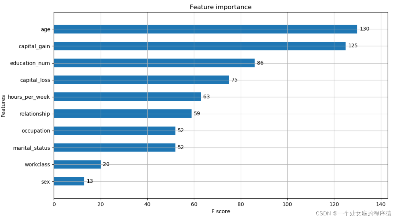
XGBR_importance_dict: [('age', 130), ('capital_gain', 125), ('education_num', 86), ('capital_loss', 75), ('hours_per_week', 63), ('relationship', 59), ('marital_status', 52), ('occupation', 52), ('workclass', 20), ('sex', 13), ('native_country', 10), ('race', 6)]
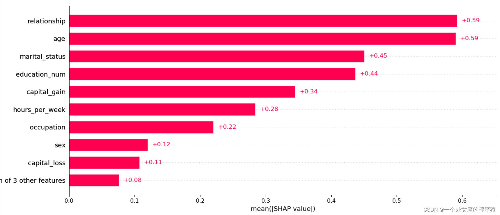
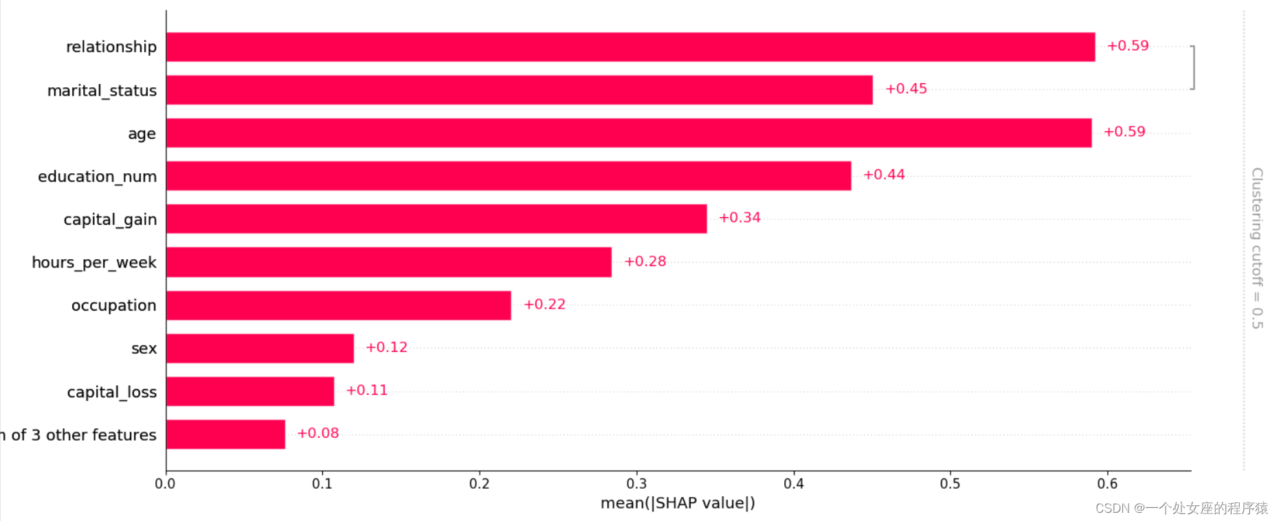
# T2、 utilize Shap Value interpretation XGBR Model
utilize shap The built-in function realizes the visualization of feature contribution —— The ranking of feature importance is similar to the above , But it's not the same
# (1)、 establish Explainer And calculate SHAP value

# T2.1、 Output shap.Explanation object
# T2,2、 Output numpy.array Array
shap2exp.values.shape (30933, 12)
 [[ 0.31074238 -0.16607898  0.5617416  ... -0.04660619 -0.09465054
   0.00530914]
 [ 0.34912622 -0.16633348  0.65308005 ... -0.06718991 -0.9804511
   0.00515459]
 [ 0.21971266  0.02263742 -0.299867   ... -0.0583196  -0.09738331
   0.00415599]
 ...
 [-0.48140627  0.07019287 -0.30844492 ... -0.04253047 -0.10924102
   0.00649792]
 [ 0.39729887 -0.2313431  -0.45257783 ... -0.06502013  0.27416423
   0.00587647]
 [ 0.27594262  0.03170239  0.78293955 ... -0.06743324  0.31613
   0.00530914]]
shap2array.shape (30933, 12)
 [[ 0.31074238 -0.16607898  0.5617416  ... -0.04660619 -0.09465054
   0.00530914]
 [ 0.34912622 -0.16633348  0.65308005 ... -0.06718991 -0.9804511
   0.00515459]
 [ 0.21971266  0.02263742 -0.299867   ... -0.0583196  -0.09738331
   0.00415599]
 ...
 [-0.48140627  0.07019287 -0.30844492 ... -0.04253047 -0.10924102
   0.00649792]
 [ 0.39729887 -0.2313431  -0.45257783 ... -0.06502013  0.27416423
   0.00587647]
 [ 0.27594262  0.03170239  0.78293955 ... -0.06743324  0.31613
   0.00530914]]
shap2exp.values And shap2array, Whether the two matrices are equal : True
# (2)、 Characteristics of the whole sample shap Value bar graph visualization
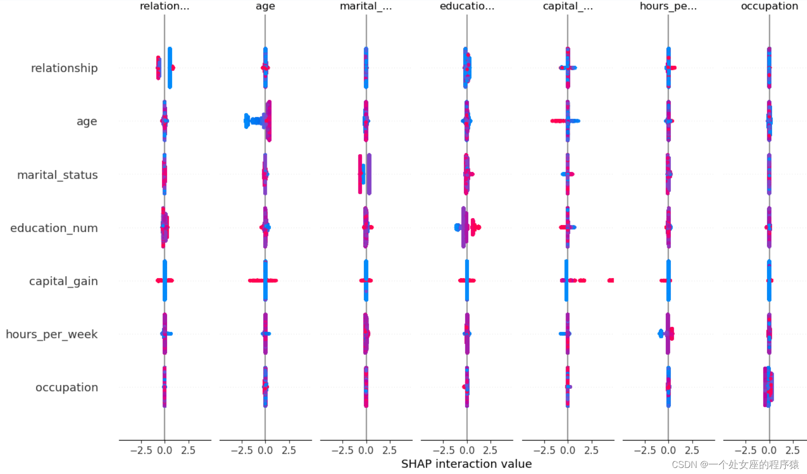
# shap Value high-order interactive visualization
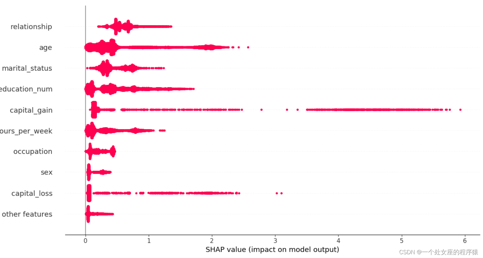
# (3)、 Characteristics of the whole sample shap Value colony graph visualization
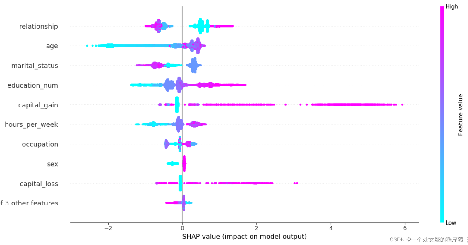
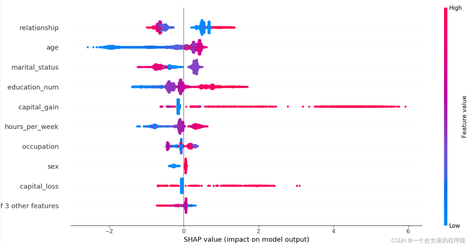
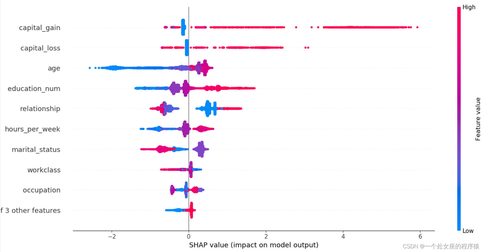
# (4)、 Global feature importance sorting scatter diagram visualization
#4.2、 Visualization of local feature importance
# (1)、 Single sample full feature bar graph visualization
Pre test samples :0
.values =
array([ 0.31074238, -0.16607898,  0.5617416 , -0.58709425, -0.08897061,
       -0.6133537 ,  0.01539118,  0.04758333, -0.3988452 , -0.04660619,
       -0.09465054,  0.00530914], dtype=float32)
.base_values =
-1.3270257
.data =
array([3.900e+01, 7.000e+00, 1.300e+01, 4.000e+00, 1.000e+00, 1.000e+00,
       4.000e+00, 1.000e+00, 2.174e+03, 0.000e+00, 4.000e+01, 3.900e+01])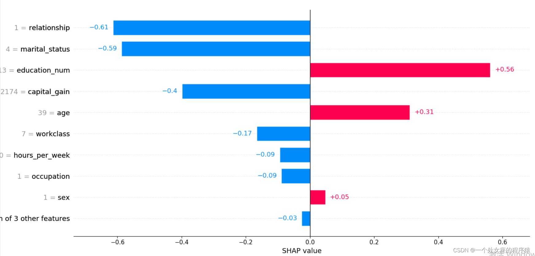
Pre test samples :1
.values =
array([ 0.34912622, -0.16633348,  0.65308005,  0.3069151 ,  0.26878497,
        0.5229906 ,  0.01030679,  0.04531586, -0.15429462, -0.06718991,
       -0.9804511 ,  0.00515459], dtype=float32)
.base_values =
-1.3270257
.data =
array([50.,  6., 13.,  2.,  4.,  0.,  4.,  1.,  0.,  0., 13., 39.])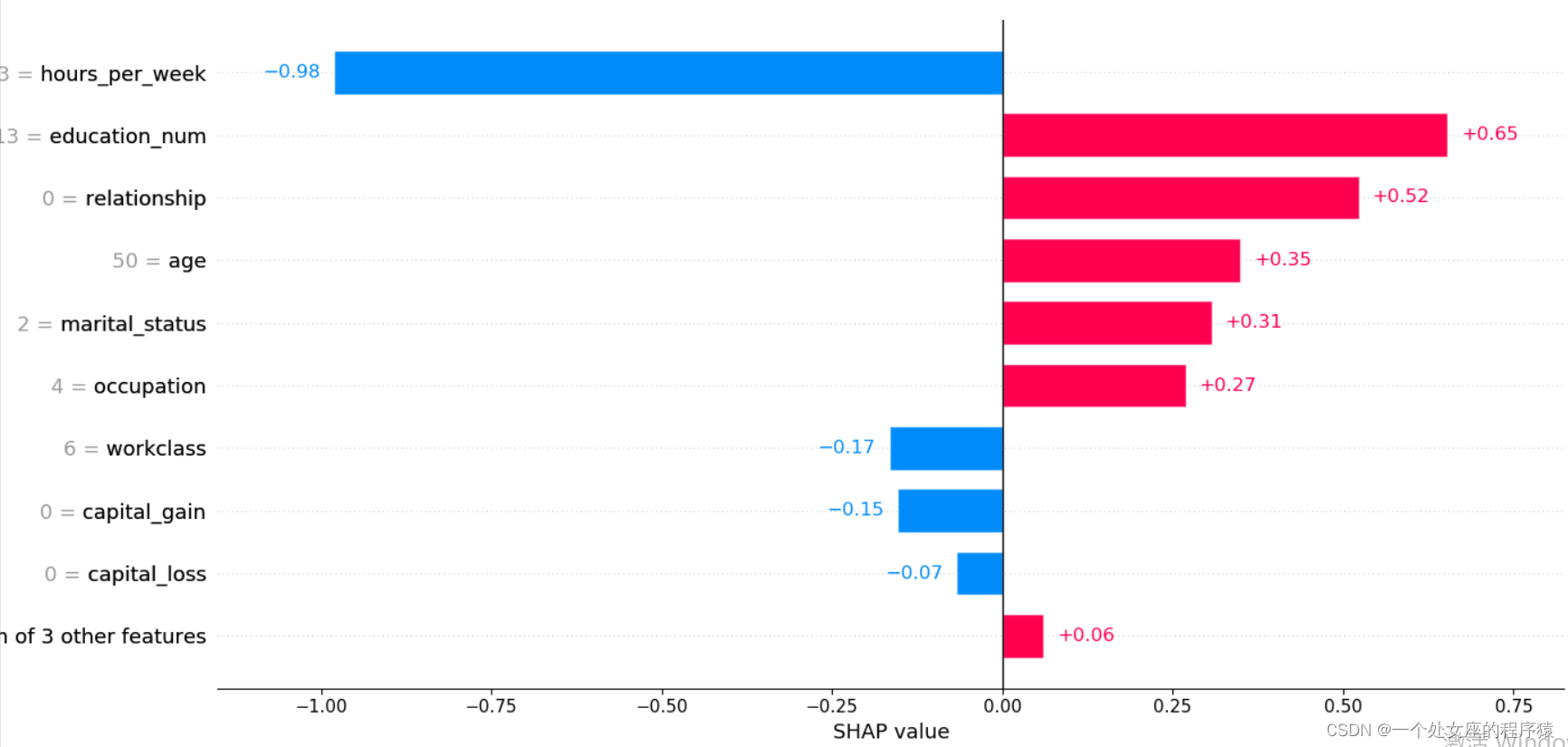
Pre test samples :10
.values =
array([ 0.27578622,  0.02686635, -0.0699547 ,  0.2820353 ,  0.3097189 ,
        0.55229187, -0.03686382,  0.05135565, -0.1607191 , -0.06321771,
        0.38190693,  0.02023092], dtype=float32)
.base_values =
-1.3270257
.data =
array([37.,  4., 10.,  2.,  4.,  0.,  2.,  1.,  0.,  0., 80., 39.])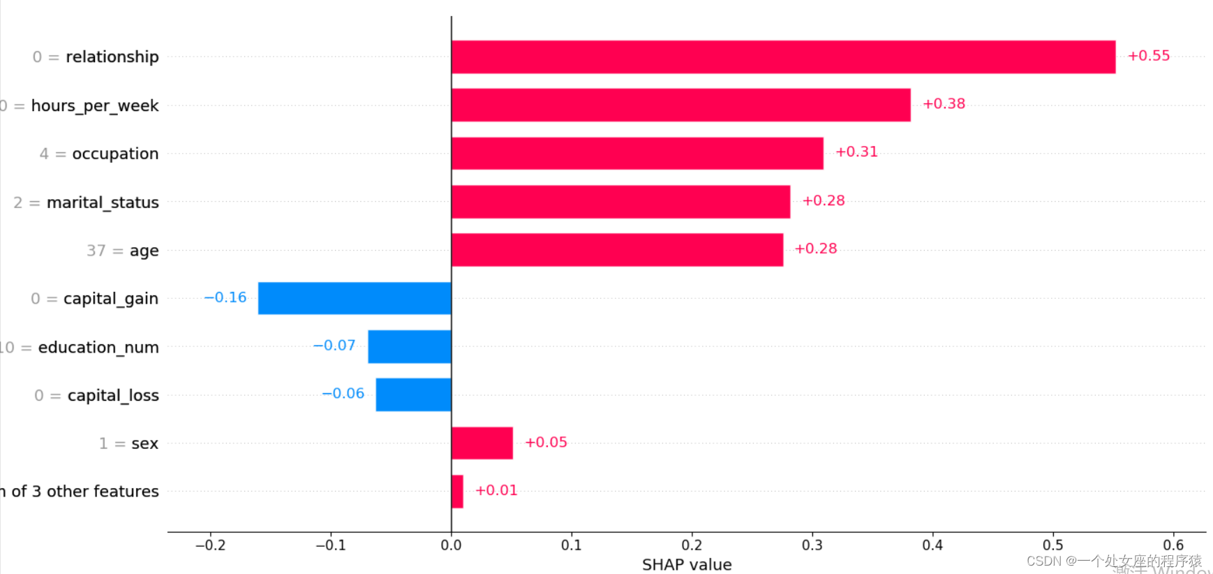
Pre test samples :20
.values =
array([ 0.31008577,  0.00316932,  1.3133987 ,  0.16768128,  0.18239255,
        0.6863757 ,  0.00508371,  0.05159741, -0.15813455, -0.06736177,
        0.31327826,  0.01936885], dtype=float32)
.base_values =
-1.3270257
.data =
array([40.,  4., 16.,  2., 10.,  0.,  4.,  1.,  0.,  0., 60., 39.])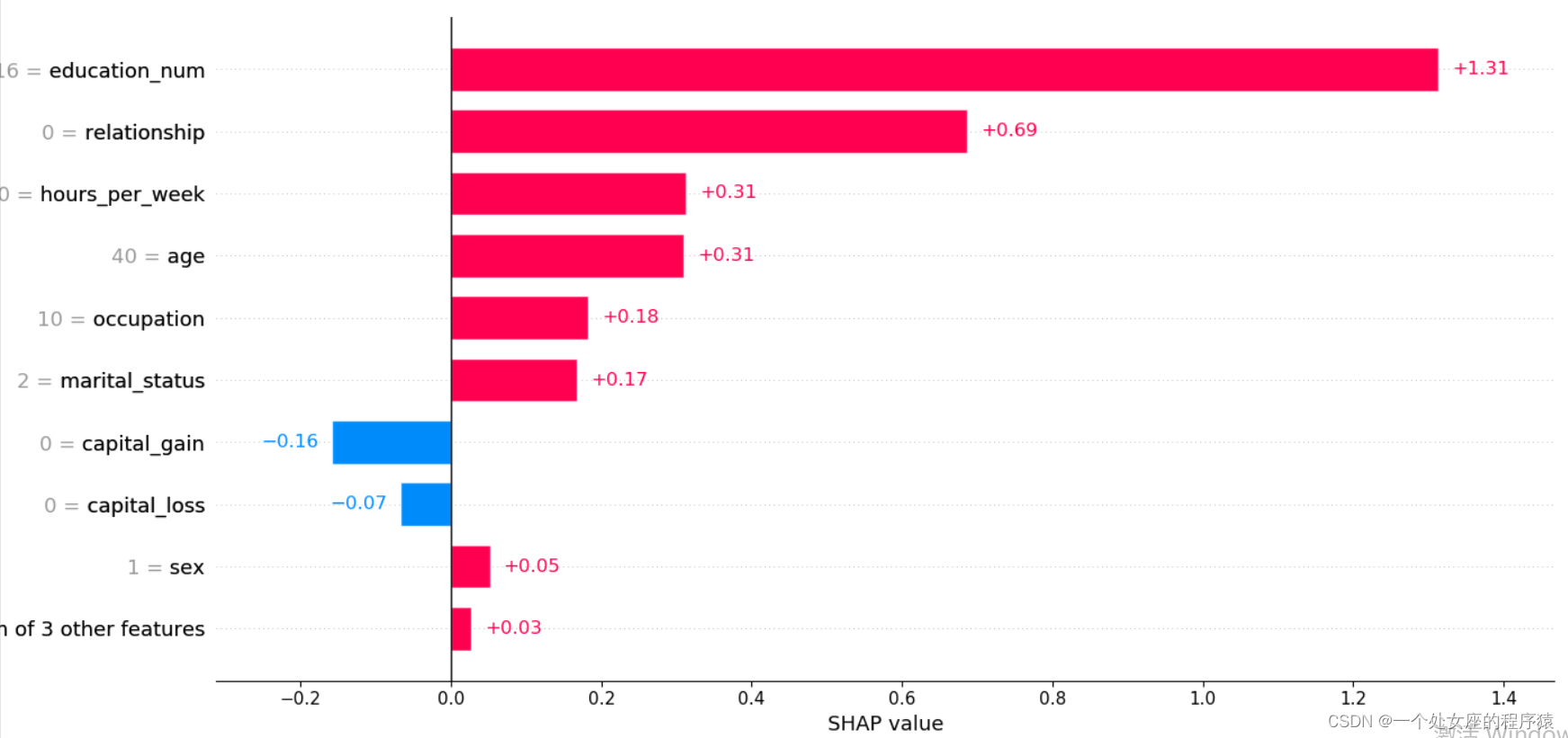
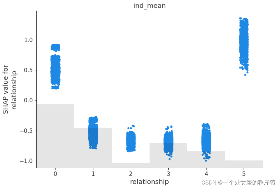
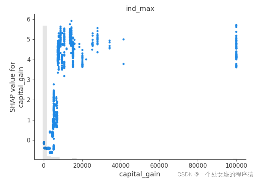
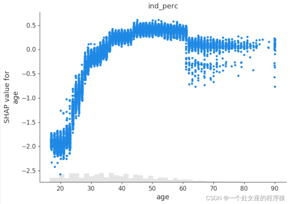
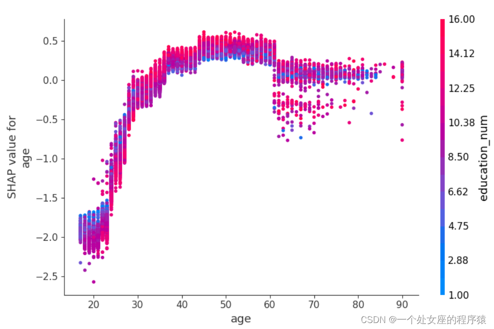
# (2)、 One turn two feature full sample local independent graph scatter diagram visualization
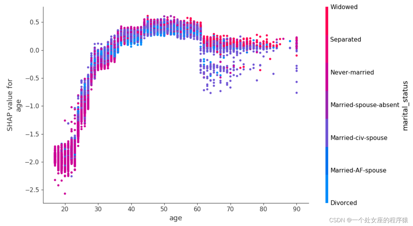
# (3)、 Visualization of double feature full sample scatter diagram
# 4.3、 Model feature screening
# (1)、 Clustering based shap Feature filtering visualization
5、 Interpretability of model prediction ( can The main Analyze misclassified samples )
Provides details of the forecast , Focus on explaining how individual forecasts are generated . It can help decision makers trust models , And explain how each feature affects the single decision of the model .
# 5.1、 Try to visualize analysis : Visualize the contribution of each feature in a single or multiple samples and Compare the predicted value of the model —— Explore misclassification samples
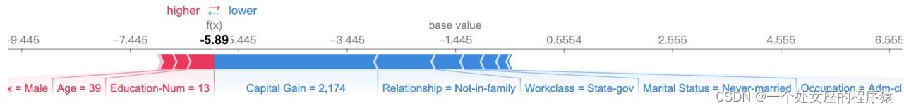
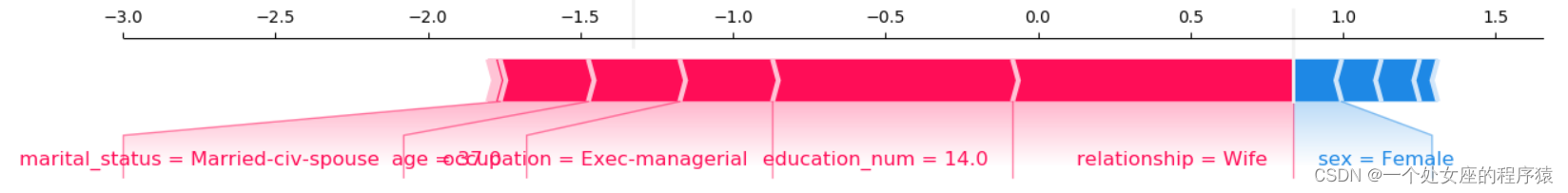
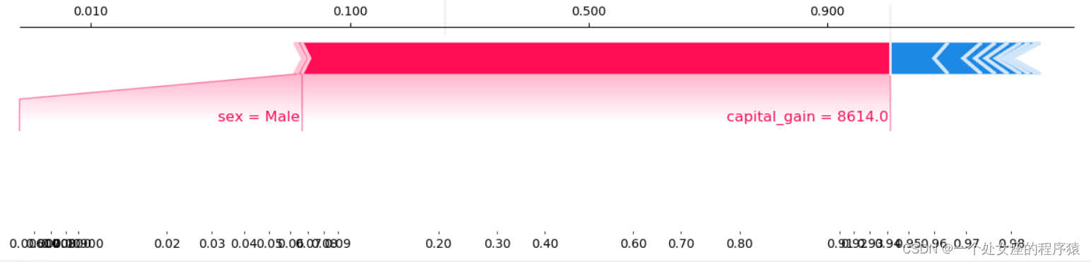
It provides the explicability of single model prediction , It can be used for error analysis , Find an explanation for the prediction of a particular instance . For example 0 Shown :
(1)、 Model output :5.89;
(2)、 Base value :base value namely explainer.expected_value, That is, the average value of model output and training data ;
(3)、 The number below the drawing arrow is the characteristic value of this instance . Such as Age=39;
(4)、 Red Indicates the Contribution is positive ( Will forecast Push up Characteristics of ), Blue Representing this feature The contribution is negative ( Will forecast PUSH low Characteristics of ). Length indicates influence ; The longer the arrow , The influence of features on output ( contribution ) The bigger it is . adopt x The scale value on the axis can see the reduction or increase of influence .
(1)、 A single sample Try to visualize — Compare predictions
Output the current test sample :0

mode_exp_value: -1.3270257
<IPython.core.display.HTML object>
 Output the current test sample :0
 age               29.0
workclass          4.0
education_num      9.0
marital_status     4.0
occupation         1.0
relationship       3.0
race               2.0
sex                0.0
capital_gain       0.0
capital_loss       0.0
hours_per_week    60.0
native_country    39.0
y_val_predi        0.0
y_val              0.0
Name: 11311, dtype: float64
 Output the true of the current test sample label: 0
 Output the prediction probability of the current test sample : 0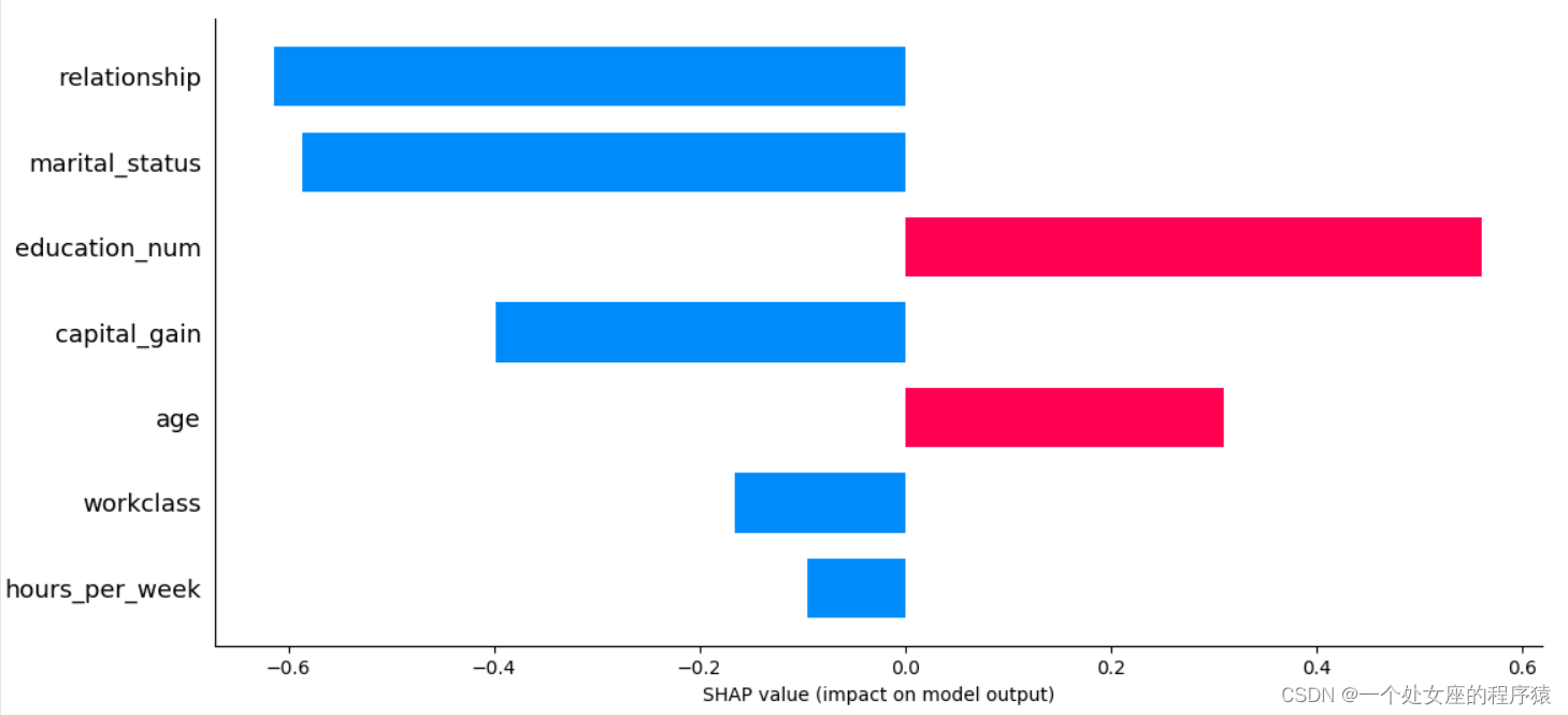
Output the current test sample :1

 Output the current test sample :1
 age                 33.0
workclass            4.0
education_num       10.0
marital_status       4.0
occupation           3.0
relationship         1.0
race                 2.0
sex                  1.0
capital_gain      8614.0
capital_loss         0.0
hours_per_week      40.0
native_country      39.0
y_val_predi          1.0
y_val                1.0
Name: 12519, dtype: float64
 Output the true of the current test sample label: 1
 Output the prediction probability of the current test sample : 1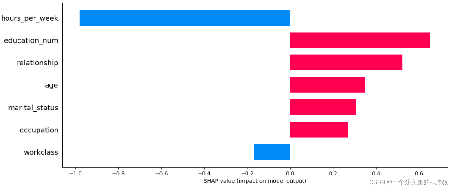
Output the current test sample :5
 Output the current test sample :5
 age               45.0
workclass          4.0
education_num     10.0
marital_status     2.0
occupation         4.0
relationship       0.0
race               4.0
sex                1.0
capital_gain       0.0
capital_loss       0.0
hours_per_week    40.0
native_country    39.0
y_val_predi        1.0
y_val              0.0
Name: 4319, dtype: float64
 Output the true of the current test sample label: 0
 Output the prediction probability of the current test sample : 1
Output the current test sample :7
 Output the current test sample :7
 age               60.0
workclass          0.0
education_num     13.0
marital_status     2.0
occupation         0.0
relationship       0.0
race               4.0
sex                1.0
capital_gain       0.0
capital_loss       0.0
hours_per_week     8.0
native_country    39.0
y_val_predi        0.0
y_val              1.0
Name: 4721, dtype: float64
 Output the true of the current test sample label: 1
 Output the prediction probability of the current test sample : 0
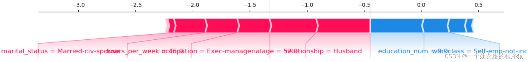
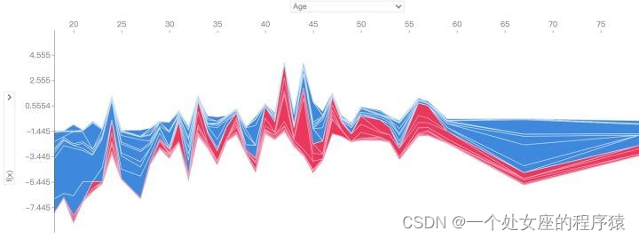
(2)、 Multiple samples Try to visualize
# (2.1)、 Visualization of feature contribution , Use the dark red and dark blue map to visualize the front 5 A prediction explanation , have access to X Data sets .
# (2.2)、 Misclassification attempts to visualize , Definitely X_val Data sets , Because it involves model prediction .
If multiple samples are interpreted , Rotate the above form 90 Degrees and then placed horizontally side by side , Get the variant of the effort
# 5.2、 Visual analysis of decision diagram : How models make decisions
# (1)、 Single sample decision Figure Visualization
# (2)、 Multiple sample decisions Figure Visualization
# (2.1)、 Visualization of some sample decision diagrams
# (2.2)、 Misclassification sample decision graph visualization
边栏推荐
- Market segmentation of supermarket customers based on purchase behavior data (RFM model)
- Phishing & filename inversion & Office remote template
- Making interactive page of "left tree and right table" based on jeecg-boot
- [English] Grammar remodeling: the core framework of English Learning -- English rabbit learning notes (1)
- Leetcode - 152 product maximum subarray
- [Yu Yue education] Dunhuang Literature and art reference materials of Zhejiang Normal University
- Chinese English comparison: you can do this Best of luck
- Is it difficult for girls to learn software testing? The threshold for entry is low, and learning is relatively simple
- 详解SQL中Groupings Sets 语句的功能和底层实现逻辑
- 【刷题】怎么样才能正确的迎接面试?
猜你喜欢
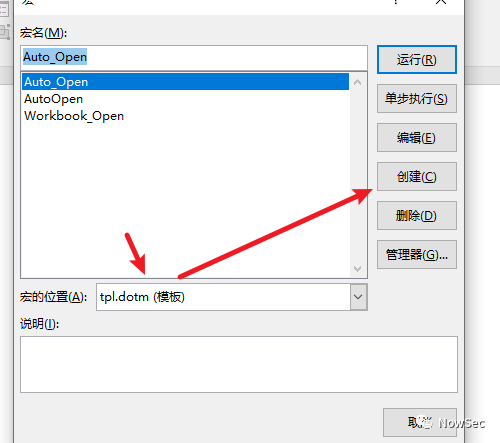
Phishing & filename inversion & Office remote template

The internationalization of domestic games is inseparable from professional translation companies

Basic commands of MySQL
![[English] Grammar remodeling: the core framework of English Learning -- English rabbit learning notes (1)](/img/02/41dcdcc6e8f12d76b9c1ef838af97d.png)
[English] Grammar remodeling: the core framework of English Learning -- English rabbit learning notes (1)

The ECU of 21 Audi q5l 45tfsi brushes is upgraded to master special adjustment, and the horsepower is safely and stably increased to 305 horsepower

How effective is the Chinese-English translation of international economic and trade contracts

My creation anniversary
![[unity] how to export FBX in untiy](/img/03/b7937a1ac1a677f52616186fb85ab3.jpg)
[unity] how to export FBX in untiy

字幕翻译中翻英一分钟多少钱?

Wish Dragon Boat Festival is happy
随机推荐
Py06 dictionary mapping dictionary nested key does not exist test key sorting
如何做好金融文献翻译?
Private cloud disk deployment
Luogu p2089 roast chicken
SQL Server Manager studio (SSMS) installation tutorial
My creation anniversary
CS-证书指纹修改
Modify the list page on the basis of jeecg boot code generation (combined with customized components)
云服务器 AccessKey 密钥泄露利用
Automated test environment configuration
Reflex WMS中阶系列3:显示已发货可换组
Wish Dragon Boat Festival is happy
雲上有AI,讓地球科學研究更省力
Grouping convolution and DW convolution, residuals and inverted residuals, bottleneck and linearbottleneck
LeetCode 1200. Minimum absolute difference
Bitcoinwin (BCW): 借贷平台Celsius隐瞒亏损3.5万枚ETH 或资不抵债
论文摘要翻译,多语言纯人工翻译
[unity] how to export FBX in untiy
On the first day of clock in, click to open a surprise, and the switch statement is explained in detail
【软件测试进阶第1步】自动化测试基础知识