当前位置:网站首页>利用超球嵌入来增强对抗训练
利用超球嵌入来增强对抗训练
2022-07-02 06:26:00 【MezereonXP】
利用超球嵌入来增强对抗训练
这次介绍一篇NeurIPS2020的工作,“Boosting Adversarial Training with Hypersphere Embedding”,一作是清华的Tianyu Pang。
该工作主要是引入了一种技术,称之为Hypersphere Embedding,本文将其称作超球嵌入。
该方法和现有的一些对抗训练的变种是正交的,即可以互相融合提升效果。
这里指的对抗训练的变种有 ALP, TRADE 等
对抗训练框架
首先,如下图所示,我们列出来AT以及其变种,用粉色标识出来其训练目标的差异
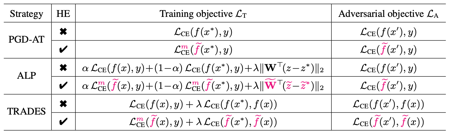
其中, x ∗ x^* x∗ 是对抗样本,右边的对抗目标可以理解为用于生成对抗样本的误差函数。
我们可以简单地看出来这些变种的设计:
- ALP是加上了正常样本的交叉熵误差,并引入了一个正则化项, z z z 其实就是 f ( x ) f(x) f(x)
- TRADES则是在引入正常样本的交叉熵误差之后,将原本的对抗样本的误差做了修改,即,从原本的标签 y y y 改为正常样本的输出 f ( x ) f(x) f(x)
HE的修改部分主要有两块:
- 在模型 f f f 上面
- 在交叉熵误差 L C E \mathcal{L}_{CE} LCE 上面
方法介绍
记号描述
这里首先给出一些基础的记号,方便后面的描述
我们考虑分类任务,记标签数量为 L L L, 记模型为:
f ( x ) = S ( W ⊤ z + b ) f(x) = \mathbb{S}(\mathbf{W}^\top z+b) f(x)=S(W⊤z+b)
其中, z = z ( x ; ω ) z = z(x;\omega) z=z(x;ω) 代表着基于模型参数 ω \omega ω 抽取出来的特征,矩阵 W = ( W 1 , . . . , W L ) \mathbf{W} = (W_1,...,W_L) W=(W1,...,WL) 以及偏置 b b b 可以理解为最后的线性层,函数 S ( ⋅ ) \mathbb{S}(\cdot) S(⋅) 是softmax函数。
我们记交叉熵误差为:
L C E ( f ( x ) , y ) = − 1 y ⊤ log f ( x ) \mathcal{L}_{CE}(f(x),y)=-1^\top_y \log f(x) LCE(f(x),y)=−1y⊤logf(x)
其中, 1 y 1_y 1y 就是标签 y y y 的 one-hot 编码,也就是在 y y y 位置上为1,其余都是0。
我们使用 ∠ ( u , v ) \angle(u,v) ∠(u,v) 表示向量 u u u 和 v v v 之间的夹角
融合HE的对抗训练框架
首先,大多数的对抗训练可以写成如下的二阶段框架:
min ω , W E [ L T ( ω , W ∣ x , x ∗ , y ) ] , where x ∗ = arg max x ′ ∈ B ( x ) L A ( x ′ ∣ x , y , ω , W ) \min_{\omega,\mathbf{W}}\mathbb{E}[\mathcal{L}_T(\omega,\mathbf{W}|x,x^*,y)], \text{where } x^*=\arg\max_{x'\in\mathbf{B}(x)} \mathcal{L}_A(x'|x,y,\omega,\mathbf{W}) ω,WminE[LT(ω,W∣x,x∗,y)],where x∗=argx′∈B(x)maxLA(x′∣x,y,ω,W)
其实就是,先生成对抗样本,然后优化训练目标。
在多次迭代之后, W \mathbf{W} W 以及 ω \omega ω 就会逐渐收敛,为了提高这种对抗训练的性能,有一些工作将metric learning引入进对抗学习之中,不过这些工作的计算代价比较高昂,会导致一些类别偏向,在更强的对抗攻击之下仍然也是脆弱的。
相关材料:
- NeurIPS 2019: Metric learning for adversarial robustness.
- IWSBPR 2015: Deep metric learning using triplet network.
- 更强的对抗攻击:https://github.com/Line290/FeatureAttack
其实这里的motivation并不充分,给的理由仍然不够有力
接下来,直接给出HE的形式,其实就是对特征 z z z 以及权重 W \mathbf{W} W 进行标准化
W ⊤ z = ( W 1 ⊤ z , W 2 ⊤ z , . . . , W L ⊤ z ) \mathbf{W}^\top z=(W_1^\top z, W_2^\top z,...,W_L^\top z) W⊤z=(W1⊤z,W2⊤z,...,WL⊤z)
其中 W i ⊤ z = ∥ W i ∥ ∥ z ∥ cos θ i W_i^\top z=\Vert W_i\Vert\Vert z\Vert \cos\theta_i Wi⊤z=∥Wi∥∥z∥cosθi, θ i = ∠ ( W i , z ) \theta_i = \angle(W_i,z) θi=∠(Wi,z)
我们令
W i ~ = W i ∥ W i ∥ , z ~ = z ∥ z ∥ \widetilde{W_i}=\frac{W_i}{\Vert W_i\Vert}, \widetilde{z}=\frac{z}{\Vert z\Vert} Wi=∥Wi∥Wi,z=∥z∥z
从而有
f ~ ( x ) = S ( W ~ ⊤ z ~ ) = cos θ θ = ( cos θ 1 , cos θ 2 , . . . , cos θ L ) \widetilde{f}(x) = \mathbb{S}(\widetilde{\mathbf{W}}^\top \widetilde{z}) = \cos\theta\\ \theta = (\cos\theta_1,\cos\theta_2,...,\cos\theta_L) f(x)=S(W⊤z)=cosθθ=(cosθ1,cosθ2,...,cosθL)
计算交叉熵函数的时候,引入一个变量 m m m,记:
L C E m ( f ~ ( x ) , y ) = − 1 y ⊤ log ( S ( s ⋅ ( cos θ − m ⋅ 1 y ) ) ) \mathcal{L}_{CE}^{m}(\widetilde{f}(x),y)=-1^\top_y\log(\mathbb{S}(s\cdot(\cos\theta-m\cdot 1_y))) LCEm(f(x),y)=−1y⊤log(S(s⋅(cosθ−m⋅1y)))
其中 s > 0 s > 0 s>0 是一个系数,用于提高训练时候的数值的稳定性
这个 m m m 的引入是参考了CVPR2018的一篇文章,Cosface: Large margin cosine loss for deep face recognition
理论分析
首先我们定义一个向量函数 U p \mathbb{U}_p Up
U p ( u ) = arg max ∥ v ∥ p ≤ 1 u ⊤ v , where u ⊤ U p ( u ) = ∥ u ∥ q \mathbb{U}_p(u)=\arg\max_{\Vert v\Vert_p\leq 1}u^\top v,\text{where } u^\top\mathbb{U}_p(u)=\Vert u\Vert_q Up(u)=arg∥v∥p≤1maxu⊤v,where u⊤Up(u)=∥u∥q
其中 1 p + 1 q = 1 \frac{1}{p}+\frac{1}{q}=1 p1+q1=1
引理1:给定一个对抗目标误差函数 L A \mathcal{L}_A LA,令 B ( x ) = { x ′ ∣ ∥ x − x ′ ∥ p ≤ ε } \mathbf{B}(x)=\{x'|\Vert x-x'\Vert_p\leq\varepsilon\} B(x)={ x′∣∥x−x′∥p≤ε},利用一阶泰勒展开,可得 max x ′ ∈ B ( x ) L A ( x ′ ) \max_{x'\in \mathbf{B}(x)}\mathcal{L}_A(x') maxx′∈B(x)LA(x′) 的解为 x ∗ = x + ε U p ( ∇ x L A ) x^*=x+\varepsilon \mathbb{U}_p(\nabla_x\mathcal{L}_A) x∗=x+εUp(∇xLA)。进一步的, L A ( x ∗ ) = L A ( x ) + ε ∥ ∇ x L A ( x ) ∥ q \mathcal{L}_A(x^*) = \mathcal{L}_A(x) + \varepsilon \Vert \nabla_x\mathcal{L}_A(x) \Vert_q LA(x∗)=LA(x)+ε∥∇xLA(x)∥q
证明:
不妨令 x ′ = x + ε v x'=x+\varepsilon v x′=x+εv,其中 ∥ v ∥ p ≤ 1 \Vert v\Vert_p\leq1 ∥v∥p≤1
从而, L A ( x ′ ) = L A ( x + ε v ) \mathcal{L}_A(x')=\mathcal{L}_A(x + \varepsilon v) LA(x′)=LA(x+εv)
在 x = x − ε v x = x - \varepsilon v x=x−εv 处进行泰勒展开,得到 L A ( x + ε v ) ≈ L A ( x ) + ε v ⊤ ( ∇ x L A ) \mathcal{L}_A(x+\varepsilon v) \approx \mathcal{L}_A(x) + \varepsilon v^\top (\nabla_x\mathcal{L}_A) LA(x+εv)≈LA(x)+εv⊤(∇xLA)
故 max x ′ ∈ B ( x ) L A ( x ′ ) = L A ( x ) + ε max ∥ v ∥ p ≤ 1 v ⊤ ∇ x L A ( x ) \max_{x'\in \mathbf{B}(x)}\mathcal{L}_A(x') = \mathcal{L}_A(x) + \varepsilon \max_{\Vert v\Vert_p\leq 1} v^\top\nabla_x \mathcal{L}_A(x) maxx′∈B(x)LA(x′)=LA(x)+εmax∥v∥p≤1v⊤∇xLA(x)
这里需要用到ICML2019 First-order Adversarial Vulnerability of Neural Networks and Input Dimension的一个结 论, 即 max δ : ∥ δ ∥ p ≤ ϵ ∣ ∂ x L ⋅ δ ∣ = ϵ ∥ ∂ x L ∥ q , 1 p + 1 q = 1 \max_{\delta:\Vert \delta\Vert_p\leq\epsilon} |\partial_x\mathcal{L}\cdot \delta| = \epsilon\Vert\partial_x\mathcal{L} \Vert_q,\frac{1}{p}+\frac{1}{q}=1 maxδ:∥δ∥p≤ϵ∣∂xL⋅δ∣=ϵ∥∂xL∥q,p1+q1=1
通过引理1,我们获得了对抗样本 x ′ x' x′ 对于损失函数 L A \mathcal{L}_A LA 的影响,同时给出了 x x x 对 x ′ x' x′ 的方向。
引理2:令 W i j = W i − W j W_{ij} = W_i-W_j Wij=Wi−Wj 为两个权重的差值, z ′ = z ( x ′ ; ω ) z' = z(x';\omega) z′=z(x′;ω) 为 x ′ x' x′ 的特征向量,便有
∇ x ′ L C E ( f ( x ′ ) , f ( x ) ) = − ∑ i ≠ j f ( x ) i f ( x ′ ) j ∇ x ′ ( W i j ⊤ z ′ ) \nabla_{x'}\mathcal{L}_{CE}(f(x'),f(x)) = -\sum_{i\neq j}f(x)_if(x')_j\nabla_{x'}(W_{ij}^\top z') ∇x′LCE(f(x′),f(x))=−i=j∑f(x)if(x′)j∇x′(Wij⊤z′)
证明:
− ∇ x ′ L C E ( f ( x ′ ) , f ( x ) ) = ∇ x ′ ( f ( x ) ⊤ log f ( x ′ ) ) = ∑ i ∈ [ L ] f ( x ) i ∇ x ′ ( log f ( x ′ ) i ) = ∑ i ∈ [ L ] f ( x ) i ∇ x ′ ( log [ exp ( W i ⊤ z ′ ) ∑ j ∈ [ L ] exp ( W j ⊤ z ′ ) ] ) = ∑ i ∈ [ L ] f ( x ) i ∇ x ′ ( W i ⊤ z ′ − log ( ∑ j ∈ [ L ] exp ( W j ⊤ z ′ ) ) ) = ∑ i ∈ [ L ] f ( x ) i ( ∇ x ′ W i ⊤ z ′ − ∇ x ′ log ( ∑ j ∈ [ L ] exp ( W j ⊤ z ′ ) ) ) = ∑ i ∈ [ L ] f ( x ) i ( ∇ x ′ W i ⊤ z ′ − 1 ∑ j ∈ [ L ] exp ( W j ⊤ z ′ ) ∇ x ′ ( ∑ j ∈ [ L ] exp ( W j ⊤ z ′ ) ) ) = ∑ i ∈ [ L ] f ( x ) i ( ∇ x ′ W i ⊤ z ′ − 1 ∑ j ∈ [ L ] exp ( W j ⊤ z ′ ) ( ∑ j ∈ [ L ] exp ( W j ⊤ z ′ ) ∇ x ′ ( W j ⊤ z ′ ) ) ) = ∑ i ∈ [ L ] f ( x ) i ( ∇ x ′ W i ⊤ z ′ − ∑ j ∈ [ L ] f ( x ′ ) j ∇ x ′ ( W j ⊤ z ′ ) ) = ∑ i ∈ [ L ] f ( x ) i ( ( 1 − f ( x ′ ) i ) ∇ x ′ W i ⊤ z ′ − ∑ j ≠ i f ( x ′ ) j ∇ x ′ ( W j ⊤ z ′ ) ) = ∑ i ∈ [ L ] f ( x ) i ( ( ∑ i ≠ j exp ( W j ⊤ z ′ ) ∑ t ∈ [ L ] exp ( W t ⊤ z ′ ) ) ∇ x ′ W i ⊤ z ′ − ∑ j ≠ i f ( x ′ ) j ∇ x ′ ( W j ⊤ z ′ ) ) = ∑ i ∈ [ L ] f ( x ) i ( ( ∑ i ≠ j exp ( W j ⊤ z ′ ) ∑ t ∈ [ L ] exp ( W t ⊤ z ′ ) ) ∇ x ′ W i ⊤ z ′ − ∑ j ≠ i exp ( W j ⊤ z ′ ) ∑ t ∈ [ L ] exp ( W t ⊤ z ′ ) ∇ x ′ ( W j ⊤ z ′ ) ) = ∑ i ∈ [ L ] f ( x ) i ( ∑ i ≠ j f ( x ′ ) j ∇ x ′ ( W i j ⊤ z ′ ) ) = ∑ i ≠ j f ( x ) i f ( x ′ ) j ∇ x ′ ( W i j ⊤ z ′ ) \begin{aligned} -\nabla_{x'}\mathcal{L}_{CE}(f(x'),f(x))&=\nabla_{x'}(f(x)^\top\log f(x'))\\ &=\sum_{i\in [L]} f(x)_i\nabla_{x'}(\log f(x')_i)\\ &=\sum_{i\in [L]}f(x)_i\nabla_{x'}(\log [\frac{\exp(W_i^\top z')}{\sum_{j\in [L]}\exp(W_j^\top z')}])\\ &=\sum_{i\in [L]}f(x)_i\nabla_{x'}(W_i^\top z' - \log(\sum_{j\in [L]}\exp(W_j^\top z')))\\ &=\sum_{i\in [L]}f(x)_i(\nabla_{x'}W_i^\top z' - \nabla_{x'}\log(\sum_{j\in [L]}\exp(W_j^\top z')))\\ &=\sum_{i\in [L]}f(x)_i(\nabla_{x'}W_i^\top z' - \frac{1}{\sum_{j\in [L]}\exp(W_j^\top z')}\nabla_{x'}(\sum_{j\in [L]}\exp(W_j^\top z')))\\ &=\sum_{i\in [L]}f(x)_i(\nabla_{x'}W_i^\top z' - \frac{1}{\sum_{j\in [L]}\exp(W_j^\top z')}(\sum_{j\in [L]}\exp(W_j^\top z')\nabla_{x'}(W_j^\top z')))\\ &=\sum_{i\in [L]}f(x)_i(\nabla_{x'}W_i^\top z' - \sum_{j\in [L]}f(x')_j\nabla_{x'}(W_j^\top z'))\\ &=\sum_{i\in [L]}f(x)_i((1-f(x')_i)\nabla_{x'}W_i^\top z' - \sum_{j\neq i}f(x')_j\nabla_{x'}(W_j^\top z'))\\ &=\sum_{i\in [L]}f(x)_i((\frac{\sum_{i\neq j}\exp(W_j^\top z')}{\sum_{t\in [L]}\exp(W_t^\top z')})\nabla_{x'}W_i^\top z' - \sum_{j\neq i}f(x')_j\nabla_{x'}(W_j^\top z'))\\ &=\sum_{i\in [L]}f(x)_i((\frac{\sum_{i\neq j}\exp(W_j^\top z')}{\sum_{t\in [L]}\exp(W_t^\top z')})\nabla_{x'}W_i^\top z' - \sum_{j\neq i}\frac{\exp(W_j^\top z')}{\sum_{t\in [L]}\exp(W_t^\top z')}\nabla_{x'}(W_j^\top z'))\\ &=\sum_{i\in [L]}f(x)_i(\sum_{i\neq j}f(x')_j\nabla_{x'}(W_{ij}^\top z'))\\ &=\sum_{i\neq j}f(x)_if(x')_j\nabla_{x'}(W_{ij}^\top z') \end{aligned} −∇x′LCE(f(x′),f(x))=∇x′(f(x)⊤logf(x′))=i∈[L]∑f(x)i∇x′(logf(x′)i)=i∈[L]∑f(x)i∇x′(log[∑j∈[L]exp(Wj⊤z′)exp(Wi⊤z′)])=i∈[L]∑f(x)i∇x′(Wi⊤z′−log(j∈[L]∑exp(Wj⊤z′)))=i∈[L]∑f(x)i(∇x′Wi⊤z′−∇x′log(j∈[L]∑exp(Wj⊤z′)))=i∈[L]∑f(x)i(∇x′Wi⊤z′−∑j∈[L]exp(Wj⊤z′)1∇x′(j∈[L]∑exp(Wj⊤z′)))=i∈[L]∑f(x)i(∇x′Wi⊤z′−∑j∈[L]exp(Wj⊤z′)1(j∈[L]∑exp(Wj⊤z′)∇x′(Wj⊤z′)))=i∈[L]∑f(x)i(∇x′Wi⊤z′−j∈[L]∑f(x′)j∇x′(Wj⊤z′))=i∈[L]∑f(x)i((1−f(x′)i)∇x′Wi⊤z′−j=i∑f(x′)j∇x′(Wj⊤z′))=i∈[L]∑f(x)i((∑t∈[L]exp(Wt⊤z′)∑i=jexp(Wj⊤z′))∇x′Wi⊤z′−j=i∑f(x′)j∇x′(Wj⊤z′))=i∈[L]∑f(x)i((∑t∈[L]exp(Wt⊤z′)∑i=jexp(Wj⊤z′))∇x′Wi⊤z′−j=i∑∑t∈[L]exp(Wt⊤z′)exp(Wj⊤z′)∇x′(Wj⊤z′))=i∈[L]∑f(x)i(i=j∑f(x′)j∇x′(Wij⊤z′))=i=j∑f(x)if(x′)j∇x′(Wij⊤z′)
在引理2之上,记 y ∗ y^* y∗ 是对抗样本 x ∗ x^* x∗ 的预测输出,其中 y ≠ y ∗ y\neq y^* y=y∗
基于一些先验的观测,通常预测输出标签的概率值(Top1 的概率)要远大于其他标签的概率值
于是有
∇ x ′ L C E ( f ( x ′ ) , f ( x ) ) ≈ − f ( x ) y f ( x ′ ) y ∗ ∇ x ′ ( W y y ∗ ⊤ z ′ ) \nabla_{x'}\mathcal{L}_{CE}(f(x'),f(x))\approx -f(x)_yf(x')_{y^*}\nabla_{x'}(W_{yy^*}^\top z') ∇x′LCE(f(x′),f(x))≈−f(x)yf(x′)y∗∇x′(Wyy∗⊤z′)
其中 W y y ∗ = W y − W y ∗ W_{yy^*}=W_y-W_{y^*} Wyy∗=Wy−Wy∗
令 θ y y ∗ ′ = ∠ ( W y y ∗ , z ′ ) \theta_{yy^*}'=\angle(W_{y y^*},z') θyy∗′=∠(Wyy∗,z′), W y y ∗ ⊤ z ′ = ∥ W y y ∗ ∥ ∥ z ′ ∥ cos ( θ y y ∗ ′ ) W_{y y^*}^\top z'=\Vert W_{y y^*}\Vert\Vert z'\Vert \cos(\theta_{y y^*}') Wyy∗⊤z′=∥Wyy∗∥∥z′∥cos(θyy∗′) 并且 W y y ∗ W_{y y^*} Wyy∗ 不依赖于 x ′ x' x′
从而,每次攻击的迭代下, x x x 的增量为
U p [ ∇ x ′ L C E ( f ( x ′ ) , f ( x ) ) ] ≈ − U p [ ∇ x ′ ( ∥ z ′ ∥ cos ( θ y y ∗ ′ ) ) ] \mathbb{U}_p[\nabla_{x'}\mathcal{L}_{CE}(f(x'),f(x))]\approx-\mathbb{U}_p[\nabla_{x'}(\Vert z'\Vert \cos(\theta_{y y^*}'))] Up[∇x′LCE(f(x′),f(x))]≈−Up[∇x′(∥z′∥cos(θyy∗′))]
而先前介绍的方法,会使得 ∥ z ′ ∥ = 1 \Vert z'\Vert = 1 ∥z′∥=1,进而使得攻击的样本更贴近分类边界
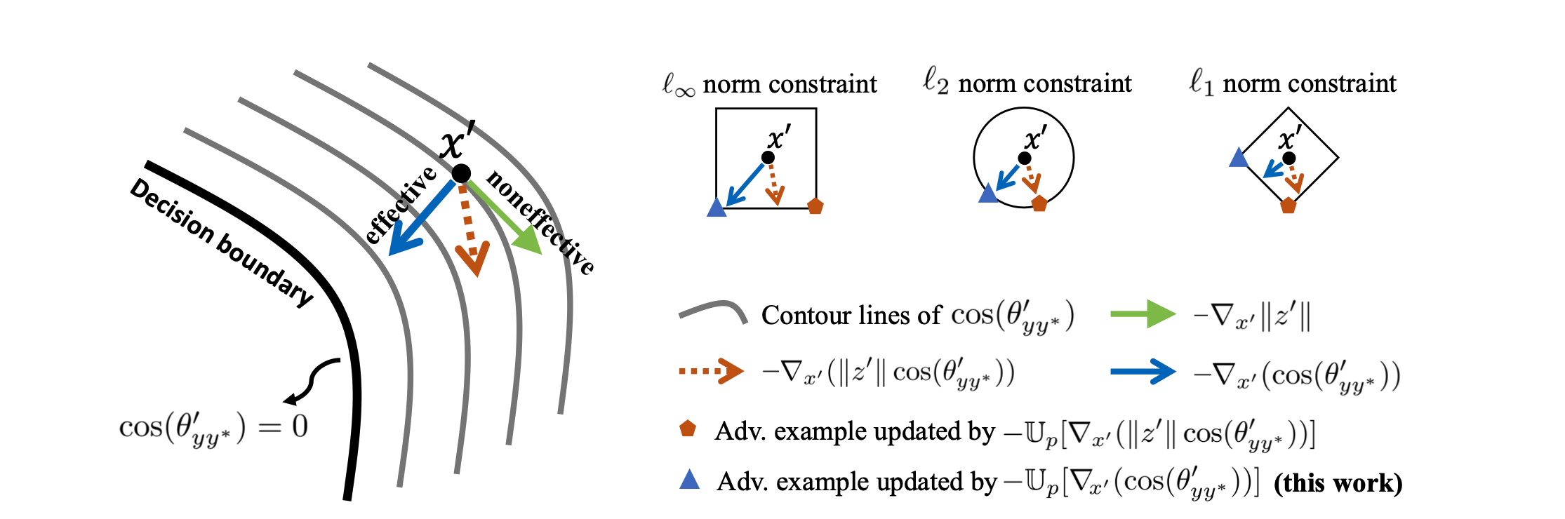
如上图所示, ∥ z ′ ∥ \Vert z'\Vert ∥z′∥ 会影响下降的方向,导致生成的对抗样本产生的作用比较差,进而抑制了对抗训练的效率
实验分析
首先是CIFAR-10上的白盒攻击测试
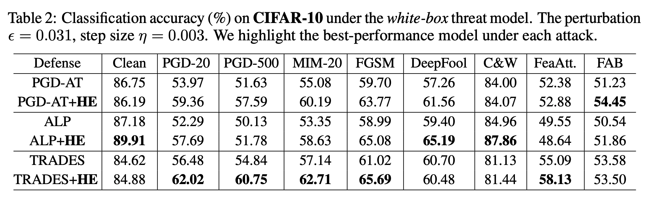
可以看到,加了HE之后防御效果会有一定的提升,少数情况下会下降
然后是ImageNet上的测试

相比FreeAT,防御效果会比较明显
边栏推荐
- Pointnet understanding (step 4 of pointnet Implementation)
- Faster-ILOD、maskrcnn_ Benchmark installation process and problems encountered
- EKLAVYA -- 利用神经网络推断二进制文件中函数的参数
- 【C#笔记】winform中保存DataGridView中的数据为Excel和CSV
- 【AutoAugment】《AutoAugment:Learning Augmentation Policies from Data》
- Semi supervised mixpatch
- 联邦学习下的数据逆向攻击 -- GradInversion
- Deep learning classification Optimization Practice
- 【学习笔记】反向误差传播之数值微分
- 图片数据爬取工具Image-Downloader的安装和使用
猜你喜欢
浅谈深度学习中的对抗样本及其生成方法
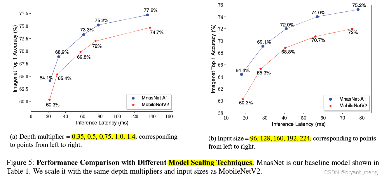
【MnasNet】《MnasNet:Platform-Aware Neural Architecture Search for Mobile》

MoCO ——Momentum Contrast for Unsupervised Visual Representation Learning
![[Sparse to Dense] Sparse to Dense: Depth Prediction from Sparse Depth samples and a Single Image](/img/05/bf131a9e2716c9147a5473db4d0a5b.png)
[Sparse to Dense] Sparse to Dense: Depth Prediction from Sparse Depth samples and a Single Image
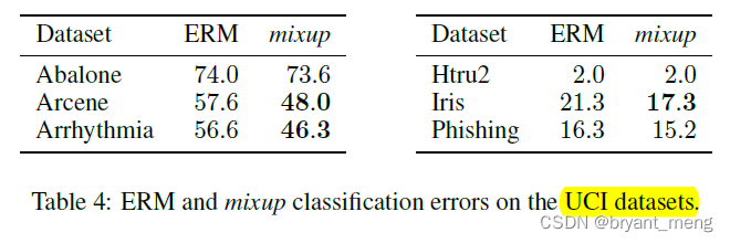
【Mixup】《Mixup:Beyond Empirical Risk Minimization》
【Mixup】《Mixup:Beyond Empirical Risk Minimization》
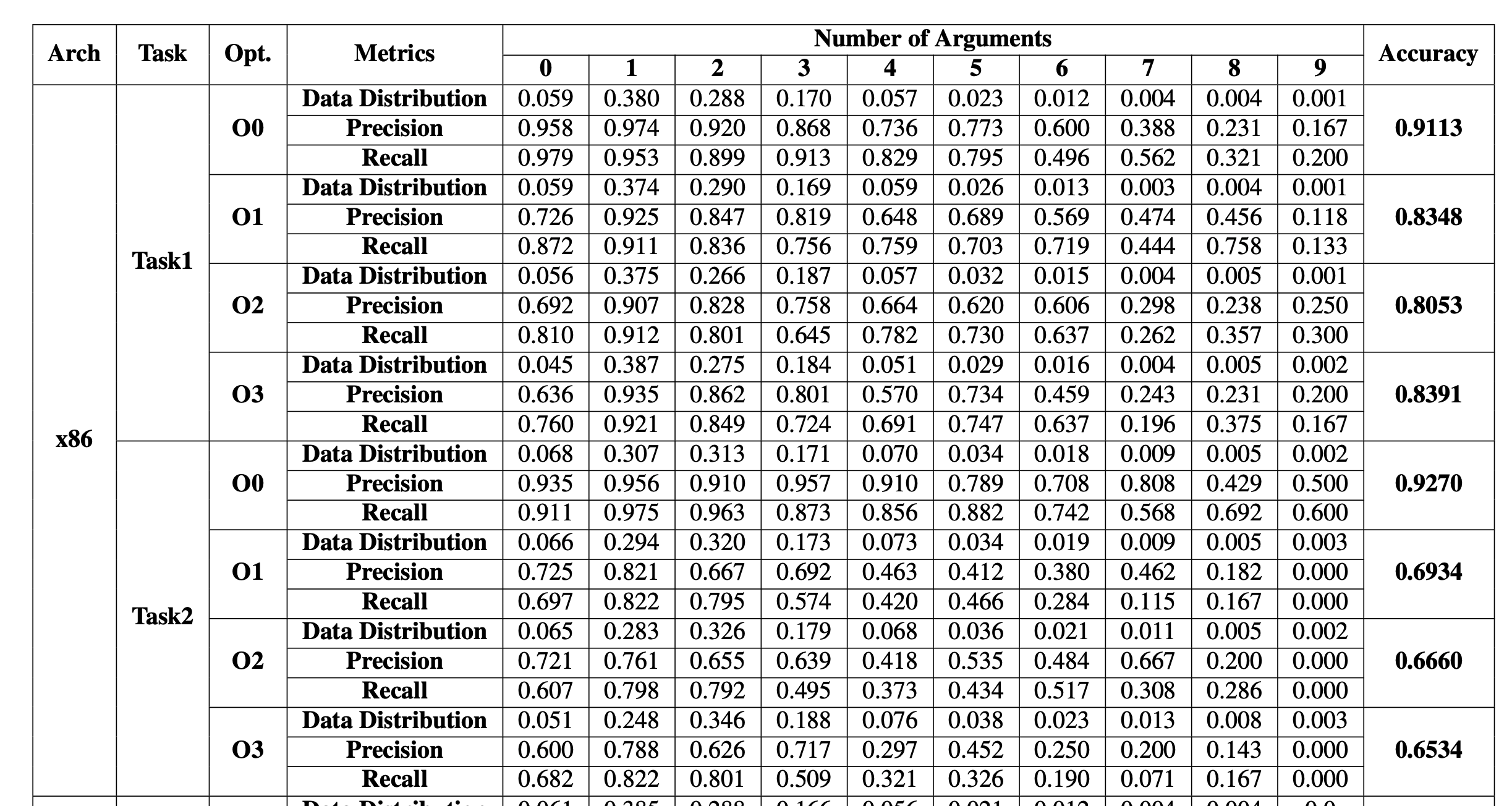
EKLAVYA -- 利用神经网络推断二进制文件中函数的参数

用MLP代替掉Self-Attention

Correction binoculaire

Implementation of yolov5 single image detection based on pytorch
随机推荐
Label propagation
Win10+vs2017+denseflow compilation
利用Transformer来进行目标检测和语义分割
深度学习分类优化实战
【Batch】learning notes
Convert timestamp into milliseconds and format time in PHP
Nacos service registration in the interface
Faster-ILOD、maskrcnn_ Benchmark trains its own VOC data set and problem summary
【TCDCN】《Facial landmark detection by deep multi-task learning》
【MnasNet】《MnasNet:Platform-Aware Neural Architecture Search for Mobile》
MMDetection安装问题
【Mixup】《Mixup:Beyond Empirical Risk Minimization》
Common machine learning related evaluation indicators
用MLP代替掉Self-Attention
EKLAVYA -- 利用神经网络推断二进制文件中函数的参数
How to turn on night mode on laptop
Generate random 6-bit invitation code in PHP
论文tips
浅谈深度学习模型中的后门
[learning notes] numerical differentiation of back error propagation