当前位置:网站首页>Several methods of image enhancement and matlab code
Several methods of image enhancement and matlab code
2022-07-02 07:58:00 【MezereonXP】
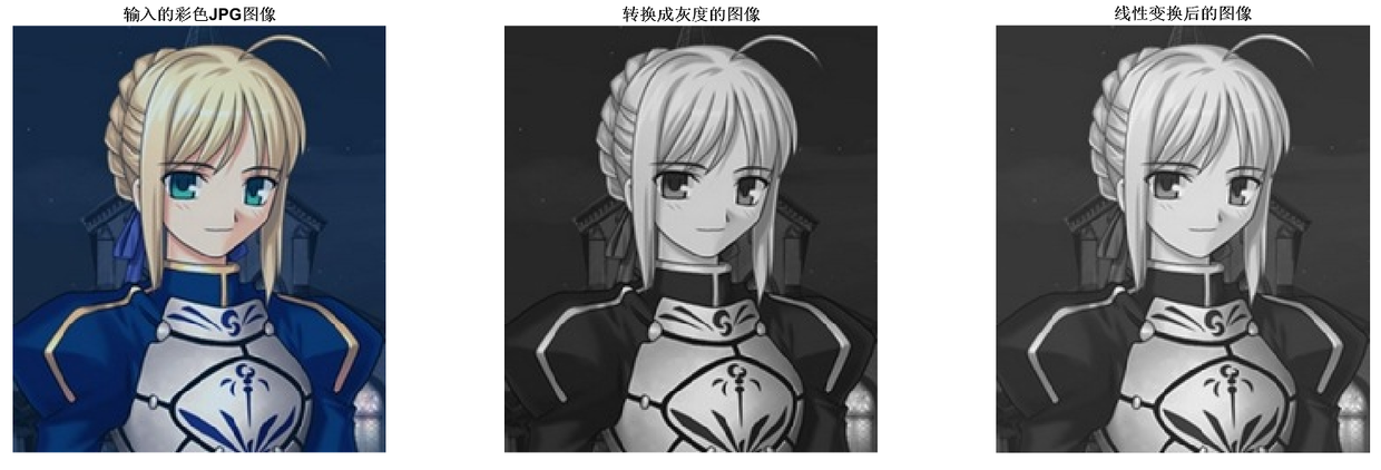
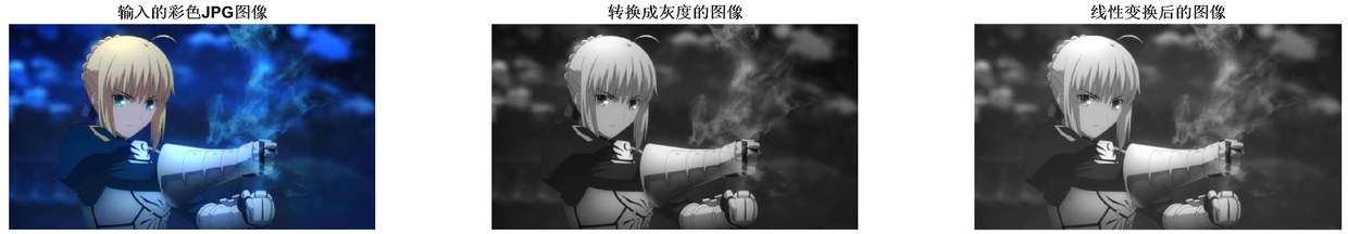
1. Gray linear transformation
Gray linear transformation , It is a method of airspace , Directly operate the gray value of each pixel
Suppose the image is I I I
Then the gray value of each pixel is I ( x , y ) I(x,y) I(x,y)
We can get :
I ( x , y ) ∗ = k ∗ I ( x , y ) + b I(x,y)^*=k*I(x,y)+b I(x,y)∗=k∗I(x,y)+b
take k = 1 , b = 16 k=1,b=16 k=1,b=16 You can get

Here are the key codes
original = imread(strcat(strcat('resource\',name),'.bmp'));
transformed = LinearFunction(original, 1, 16);
subplot(1,3,3);
imshow(transformed)
title(' Image after linear transformation ')
imwrite(transformed,strcat(strcat('result\',name),'(linear).jpg'))
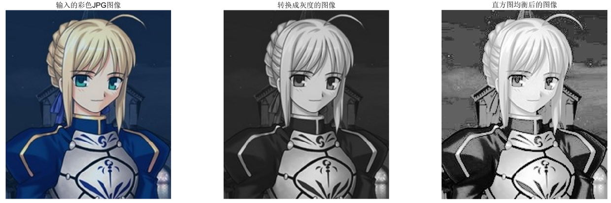
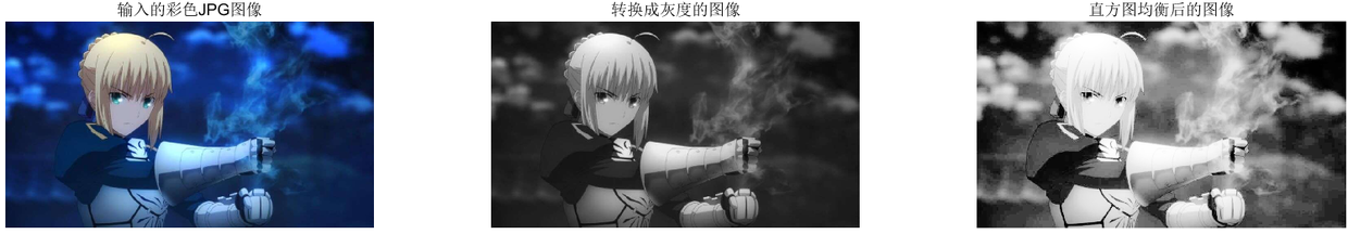
2. Histogram equalization transform
This method is usually used to increase the global contrast of many images , Especially when the contrast of the useful data of the image is quite close . In this way , Brightness can be better distributed on histogram . This can be used to enhance the local contrast without affecting the overall contrast , Histogram equalization can achieve this function by effectively expanding the commonly used brightness .
This method is very useful for both background and foreground images that are too bright or too dark , This method, in particular, can bring about X Better display of bone structure in light images and better details in overexposed or underexposed photos . One of the main advantages of this method is that it is a fairly intuitive technology and reversible operation , If the equalization function is known , Then we can restore the original histogram , And the amount of calculation is not big . One disadvantage of this method is that it does not select the data to be processed , It may increase the contrast of background noise and decrease the contrast of useful signals .
Consider a discrete grayscale image { x } \{x\} { x}
Give Way n i n_i ni Indicates grayscale i i i Number of occurrences , So the grayscale of the image is i i i The probability of pixels appearing is :
p x ( i ) = p ( x = i ) = n i n , 0 ≤ i < L p_x(i)=p(x=i)=\frac{n_i}{n}, 0\leq i<L px(i)=p(x=i)=nni,0≤i<L
L L L Is the number of grayscale in the image ( Usually 255)
Corresponding to p x p_x px The cumulative distribution function of , Defined as :
c d f x ( i ) = ∑ j = 0 i p x ( j ) cdf_x(i)=\sum_{j=0}^i{p_x(j)} cdfx(i)=∑j=0ipx(j)
Is the cumulative normalized histogram of the image
We create a form of y = T ( x ) y=T(x) y=T(x) Transformation of , For each value of the original image, it generates a y y y, such y y y The cumulative probability function of can be linearized in all value ranges , The conversion formula is defined as :
c d f y ( i ) = i K cdf_y(i)=iK cdfy(i)=iK
For constants K, C D F CDF CDF The nature of allows us to make such transformations , Defined as :
c d f y ( y ′ ) = c d f y ( T ( k ) ) = c d f x ( k ) cdf_y(y')=cdf_y(T(k))=cdf_x(k) cdfy(y′)=cdfy(T(k))=cdfx(k)
among k ∈ [ 0 , L ) k\in [0,L) k∈[0,L), Be careful T T T Map different gray levels to ( 0 , 1 ) (0,1) (0,1), To map these values to the original domain , You need to apply the following simple transformation to the result :
y ′ = y ∗ ( m a x { x } − m i n { x } ) + m i n { x } y' = y*(max\{x\}-min\{x\})+min\{x\} y′=y∗(max{ x}−min{ x})+min{ x}
Give some results :

Give the key code :
m = 255;
subplot(1,3,3);
H = histeq(I,m);
imshow(H,[]);
title(‘ Image after histogram equalization ’);
Similarly , We can rgb Image histogram equalization , Here is the result


[M,N,G]=size(I1);
result=zeros(M,N,3);
% Get every point of every layer RGB value , And determine its value
for g=1:3
    A=zeros(1,256);
    % After each layer , The parameter should be reinitialized to 0
    average=0;
    for k=1:256
        count=0;
        for i=1:M
            for j=1:N
                value=I1(i,j,g);
                if value==k
                    count=count+1;
                end
            end
        end
        count=count/(M*N*1.0);
        average=average+count;
        A(k)=average;
    end
    A=uint8(255.*A+0.5);
    for i=1:M
        for j=1:N
            I1(i,j,g)=A(I1(i,j,g)+0.5);
        end
    end
end
% Show the treatment effect
subplot(1,3,3);
imshow(I1);
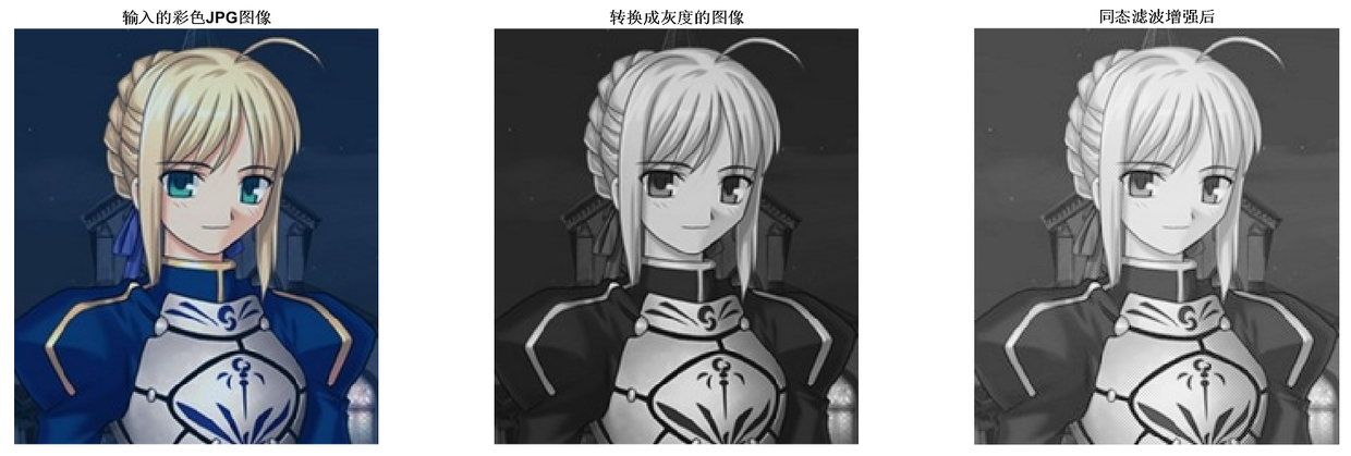
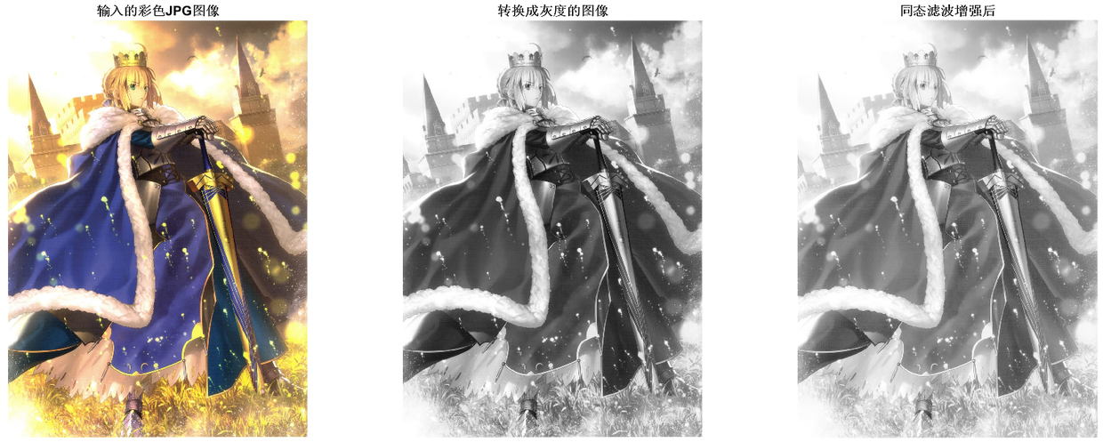
3. Homomorphic filtering
Homomorphic filtering is used to remove Multiplicative noise (multiplicative noise), It can increase contrast and standardize brightness at the same time , So as to achieve the purpose of image enhancement .
An image can be represented as its Intensity of illumination (illumination) Weight and Reflection (reflectance) The product of components , Although the two are inseparable in the time domain , But through Fourier transform, the two can be linearly separated in the frequency domain . Since the illuminance can be regarded as the lighting in the environment , The relative change is very small , It can be regarded as the low-frequency component of the image ; The reflectivity changes relatively large , It can be regarded as a high-frequency component . The influence of illuminance and reflectivity on pixel gray value is processed respectively , Usually by High pass filter (high-pass filter), Make the lighting of the image more uniform , Achieve the purpose of enhancing the detailed features of the shadow area .
It is :
For an image , It can be expressed as the product of illumination component and reflection component , That is to say :
m ( x , y ) = i ( x , y ) ⋅ r ( x , y ) m(x,y)=i(x,y)\cdot r(x,y) m(x,y)=i(x,y)⋅r(x,y)
among , m m m It's an image , i i i Is the illuminance component , r r r Is the reflection component
In order to use high pass filter in frequency domain , We have to do Fourier transform , But because the above formula is a product , It is not possible to directly operate the illumination component and reflection component , So take the logarithm of the above formula
l n ( m ( x , y ) ) = l n ( i ( x , y ) ) + l n ( r ( x , y ) ) ln(m(x,y))=ln(i(x,y))+ln(r(x,y)) ln(m(x,y))=ln(i(x,y))+ln(r(x,y))
Then Fourier transform the above formula
F { l n ( m ( x , y ) ) } = F { l n ( i ( x , y ) ) } + F { l n ( r ( x , y ) ) } \mathcal{F}\{ln(m(x,y))\}=\mathcal{F} \{ ln(i(x,y))\}+ \mathcal{F}\{ln(r(x,y))\} F{ ln(m(x,y))}=F{ ln(i(x,y))}+F{ ln(r(x,y))}
We will F { l n ( m ( x , y ) ) } \mathcal{F}\{ln(m(x,y))\} F{ ln(m(x,y))} Defined as M ( u , v ) M(u,v) M(u,v)
Next, high pass filter the image , In this way, the illumination of the image can be more uniform , The high-frequency component increases and the low-frequency component decreases
N ( u , v ) = H ( u , v ) ⋅ M ( u , v ) N(u,v)=H(u,v)\cdot M(u,v) N(u,v)=H(u,v)⋅M(u,v)
among H H H It's a high pass filter
In order to transfer the image from the frequency domain back to the time domain , We are right. N N N Do inverse Fourier transform
n ( x , y ) = F − 1 { N ( x , y ) } n(x,y)=\mathcal{F}^{-1}\{N(x,y)\} n(x,y)=F−1{ N(x,y)}
Finally, use the exponential function to restore the logarithm we took at the beginning
m ′ ( x , y ) = e x p { n ( x , y ) } m'(x,y)=exp\{n(x,y)\} m′(x,y)=exp{ n(x,y)}
The results are given

Give some key codes
I=double(I);
[M,N]=size(I);
rL=0.5;
rH=4.7;% The parameters can be adjusted according to the desired effect
c=2;
d0=10;
I1=log(I+1);% Take the logarithm
FI=fft2(I1);% The Fourier transform
n1=floor(M/2);
n2=floor(N/2);
H = ones(M, N);
for i=1:M
    for j=1:N
        D(i,j)=((i-n1).^2+(j-n2).^2);
        H(i,j)=(rH-rL).*(exp(c*(-D(i,j)./(d0^2))))+rL;% Gaussian homomorphic filtering
    end
end
I2=ifft2(H.*FI);% Inverse Fourier transform
I3=real(exp(I2));
subplot(1,3,3),imshow(I3,[]);title(' After homomorphic filtering is enhanced ');
边栏推荐
- 【DIoU】《Distance-IoU Loss:Faster and Better Learning for Bounding Box Regression》
- What if a new window always pops up when opening a folder on a laptop
- Embedding malware into neural networks
- 【TCDCN】《Facial landmark detection by deep multi-task learning》
- 【Sparse-to-Dense】《Sparse-to-Dense:Depth Prediction from Sparse Depth Samples and a Single Image》
- 【Cutout】《Improved Regularization of Convolutional Neural Networks with Cutout》
- WCF更新服务引用报错的原因之一
- 包图画法注意规范
- Gensim如何冻结某些词向量进行增量训练
- 【Batch】learning notes
猜你喜欢
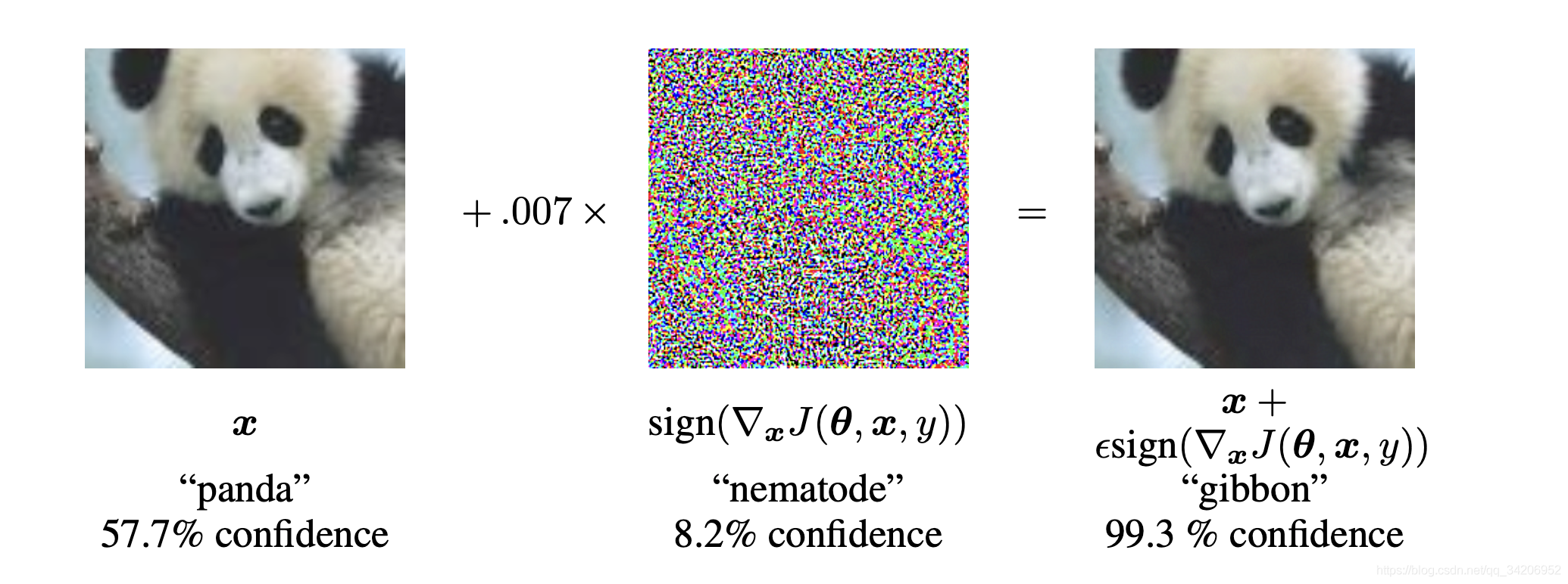
浅谈深度学习中的对抗样本及其生成方法
Semi supervised mixpatch

【Random Erasing】《Random Erasing Data Augmentation》
Feature Engineering: summary of common feature transformation methods

【DIoU】《Distance-IoU Loss:Faster and Better Learning for Bounding Box Regression》

【FastDepth】《FastDepth:Fast Monocular Depth Estimation on Embedded Systems》
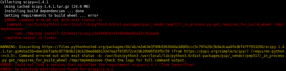
jetson nano安装tensorflow踩坑记录(scipy1.4.1)

Translation of the paper "written mathematical expression recognition with bidirectionally trained transformer"
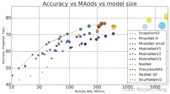
【MobileNet V3】《Searching for MobileNetV3》

Correction binoculaire
随机推荐
Command line is too long
【Hide-and-Seek】《Hide-and-Seek: A Data Augmentation Technique for Weakly-Supervised Localization xxx》
【DIoU】《Distance-IoU Loss:Faster and Better Learning for Bounding Box Regression》
【DIoU】《Distance-IoU Loss:Faster and Better Learning for Bounding Box Regression》
Remplacer l'auto - attention par MLP
C#与MySQL数据库连接
针对语义分割的真实世界的对抗样本攻击
Target detection for long tail distribution -- balanced group softmax
关于原型图的深入理解
The hystrix dashboard reported an error hystrix Stream is not in the allowed list of proxy host names solution
用MLP代替掉Self-Attention
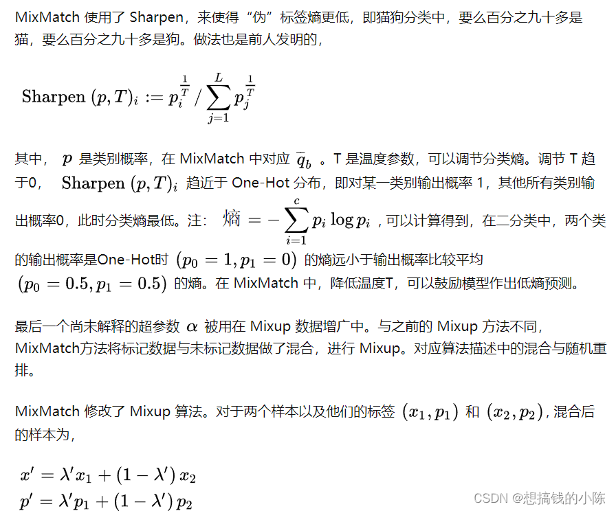
半监督之mixmatch
open3d学习笔记三【采样与体素化】
Specification for package drawing
ABM thesis translation
利用Transformer来进行目标检测和语义分割
论文tips
浅谈深度学习模型中的后门
What if the laptop can't search the wireless network signal
【Wing Loss】《Wing Loss for Robust Facial Landmark Localisation with Convolutional Neural Networks》