[statistical learning methods] learning notes - Chapter 5: Decision Tree

Decision tree （decision tree） It is a basic classification and regression method . The main advantage is that the model is readable , Fast classification . Decision tree learning usually consists of three steps ： feature selection 、 Generation of decision tree and pruning of decision tree .

1. Decision tree model and learning

1.1 Decision tree model

Definition ： Decision tree Classification decision tree model is a kind of tree structure that describes the classification of instances . The decision tree consists of nodes （node） And the directed side （directed edge） form . There are two types of nodes ： Internal nodes （internal node） And leaf nodes （leaf node）. Internal node represents a feature or attribute , A leaf node represents a class .

1.2 Decision tree and if-then The rules

Each path from the root node to the leaf node of the decision tree constructs a rule ： The characteristics of the internal nodes of the path correspond to the conditions of the rules , The class of leaf node corresponds to the conclusion of rule .
Path of decision tree or its corresponding if-then Rule set has an important property ： Mutually exclusive and complete . in other words , Every instance is covered by a path or a rule , And only covered by one path or one rule .

1.3 Decision tree and conditional probability distribution

The decision tree also represents the conditional probability distribution of a class under a given characteristic condition , This conditional probability distribution is defined in a partition of the feature space （partition） On , Dividing feature space into disjoint elements （cell） Or area （region）, And defining a class probability distribution in each unit constitutes a conditional probability distribution .
A path of the decision tree corresponds to a unit in the partition . The conditional probability distribution represented by the decision tree is composed of the conditional probability distribution of the class under the given conditions of each unit . Leaf nodes （ unit ） The conditional probability on tends to favor a certain class , That is, the probability of belonging to a certain class is high .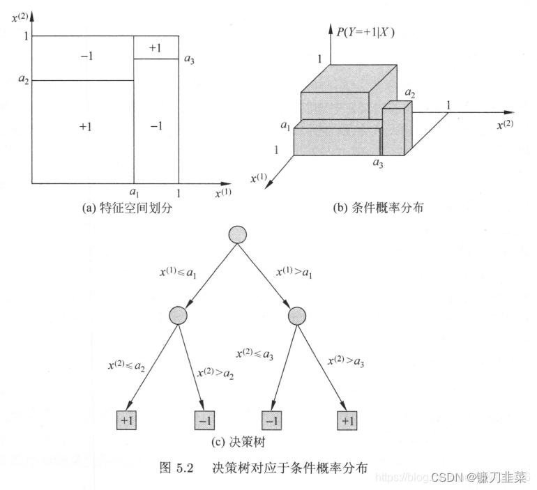

1.4 Decision tree learning

Suppose a given training data set $D=\{(x_1,y_1),(x_2,y_2),\cdots ,(x_N,y_N)\}$, among ,$x_i=(x_i^1,x_i^2,\cdots ,x_i^n{)}^T$ Enter an instance for ( Eigenvector ),$n$ For the number of features ,$y_i\in \{1,2,\cdots ,K\}$ Tag for class ,$i=1,2,\cdots ,N$,$N$ Is sample size .
Decision tree learning The goal is yes Build a decision tree model according to the given training data , It can classify instances correctly .

Decision tree learning The essence On is A set of classification rules are summarized from the training data . There may be more than one decision tree that can correctly classify the training data , Or maybe none of them . We need a decision tree with less contradiction with the training data , meanwhile Good generalization ability .

Decision tree learning Use the loss function to express this goal . Loss function of decision tree learning It is usually a regularized maximum likelihood function . The strategy of decision tree learning is Minimization with loss function as objective function .

When the loss function is determined , The learning problem becomes the problem of selecting the optimal decision tree in the sense of loss function .

Decision tree learning The algorithm is usually a recursive selection of optimal features , The training data are segmented according to this feature , The process of making the best classification of each sub data set . This process corresponds to the division of feature space , It also corresponds to the construction of decision tree .

• Start , Build the root node , Put all training data in the root node . Choose an optimal feature , According to this feature, the training data is divided into subsets , Make each subset have the best classification under the current conditions .
• If these subsets can be classified basically correctly , Then build leaf nodes , Divide these subsets into corresponding leaf nodes ;
• If there are subsets that cannot be classified basically correctly , Then select new optimal features for these subsets , Continue to split it , Build the corresponding node .
• If you go on recursively , Until all training data subsets are basically correctly classified , Or no suitable characteristics . This generates a decision tree .

The decision tree generated by the above method may have a good classification ability for the training data , but It may not have a good classification ability for unknown test data , That is, fitting phenomenon may have occurred . We need to Prune the generated tree from bottom to top , Make the tree simpler , So that it has better generalization ability .

If There are many features , Or at the beginning of decision tree learning , Select features , Only features with sufficient classification ability for training data are left .

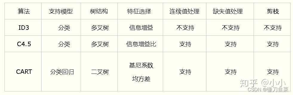
It can be seen that , Decision tree learning algorithm includes feature selection 、 The generation of decision tree and the pruning process of decision tree . Common algorithms for decision tree learning are ID3、C4.5 And CART.

2. feature selection

2.1 Feature selection problem

Feature selection is to select features with classification ability for training data . This can improve the efficiency of decision tree learning . If using a feature for classification results and random classification results are not very different , It is said that this feature has no classification ability . Generally, the criterion of feature selection is Information gain or Information gain ratio .

2.2 Information gain

In information theory and probability statistics , entropy （entropy） Is a measure of the uncertainty of a random variable . set up X Is a discrete random variable with finite values , The probability distribution is ：
$$P(X=x_i)=p_i,i=1,2,...,n$$
Then the random variable X Entropy is defined as ：
$$H(X)=-\sum _{i=1}^n{p}_i\log p_i$$
if $p_i=0$, The definition is $0\log 0=0$. Usually logarithms are expressed in 2 To base or base on e Bottom （ Natural logarithm ）, The units of entropy are called bits （bit） Or Nate （nat）.
By definition , Entropy only depends on X The distribution of , And with the X The value of has nothing to do with , So you can also X The entropy of $H(p)$, namely
$$H(p)=-\sum _{i=1}^n{p}_i\log p_i$$
The greater the entropy , The greater the uncertainty of random variables . Verifiable from definition ：
$$0\le H(p)\le \log n$$
When a random variable takes only two values , for example 1,0 when , The distribution of is ：
$$P(X=1)=p,P(X=0)=1-p,0\le p\le 1$$
The entropy is ：
$$H(p)=-p{\log }_{2}p-(1-p){\log }_2(1-p)$$
At this time , entropy $H(p)$ Random probability $p$ The curve of is shown in the figure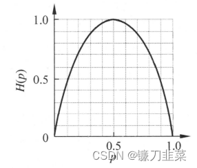

When $p=0$ or $p=1$ when $H(p)=0$, Random variables have no uncertainty at all . When $p=0.5$ when ,$H(p)=1$ , Entropy is the maximum , The random variable has the greatest uncertainty .

Conditional entropy (conditional entropy)$H(Y|X)$ I have a random variable $X$ Is a random variable $Y$ uncertainty .$H(Y|X)$ Defined as $X$ Given the conditions $Y$ The entropy pair of the conditional probability distribution $X$ Mathematical expectation
$$H(Y|X)=\sum _{i=1}^n{p}_{i}H(Y|X=x_i)$$
here $p_i=P(X=x_i),i=1,2,...,n$.

When the probability in entropy and conditional entropy is obtained by maximum likelihood estimation , The corresponding entropy and conditional entropy are called Experience in entropy (empirical entropy) and Empirical condition entropy (empirical conditional entropy). here , If by 0 probability , Then order $0\log 0=0$.

Information gain （information gain） Express To learn that feature X The information that makes the class Y The degree to which the uncertainty of information is reduced .
Definition （ Information gain ）： features $A$ On the training data set $D$ Information gain of $g(D,A)$ Defined as a set $D$ The experience of the entropy $H(D)$ With the characteristics of $A$ Given the conditions $D$ Entropy of empirical conditions $H(D|A)$ The difference between the , namely
$$g(D,A)=H(D)-H(D|A)\text{\hspace{1em}(5.6)}$$

In a general way , entropy $H(Y)$ And condition entropy $H(Y|X)$ The difference is called Mutual information (mutual information). The information gain in decision tree learning is equivalent to the mutual information of class and feature in training data set .
Decision tree learning applies information gain criteria to select features ： Given training set $D$ And characteristics $A$, Experience in entropy $H(D)$ Represents a pair of data sets $D$ The uncertainty of classification . And empirical conditional entropy $H(D|A)$ It means in the feature $A$ Given the conditions for the dataset $D$ The uncertainty of classification . So their difference , Information gain , It means that due to the characteristics $A$ And make the data set $D$ The degree to which the uncertainty of classification is reduced . obviously , Information gain depends on features , Different features often have different information gain . Features with large information gain have stronger classification ability .

Then we get the feature selection method according to the information gain criterion ： On the training data set ( Or subset )$D$, Calculate the information gain of each feature , And compare their sizes , Select the feature with maximum information gain .

Algorithm （ Algorithm of information gain ）：
Input ： Training data set D And characteristics A;
Output ： features A On the training data set D Information gain of $g(D,A)$.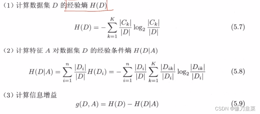

2.3 Information gain ratio

Take information gain as the feature of dividing training data set , There is a problem of choosing more features . Use Information gain ratio （information gain ratio） This problem can be corrected .
Definition （ Information gain ratio ）： features A On the training data set D The information gain ratio of $g_R(D,A)$ Defined as its information gain $g(D,A)$ With training datasets D About the characteristics of A The entropy of the value of $H_A(D)$ The ratio of the , namely ：
$$g_R(D,A)=\frac{g(D,A)}{H_A(D)}$$
among ,$H_A(D)=-{\sum }_{i=1}^n\frac{|D_i|}{D}{\log }_2\frac{|D_i|}{D}$,n Is the characteristic A Number of values .

3. Decision tree generation

3.1 ID3 Algorithm

ID3 The core of the algorithm is to apply the information gain criterion to select features on each node of the decision tree , Build the decision tree recursively . The way to do it is ： From the root node （root node） Start , Calculate the information gain of all possible features for nodes , The feature with the largest information gain is selected as the feature of the node , The sub nodes are established according to the different values of the feature ; Then call the above method recursively to the child node , Build decision tree ; Until the information gain of all features is very small or no features can be selected , Finally, a decision tree is obtained .ID3 It's equivalent to using the maximum likelihood method to select the probability model .
Algorithm （ID3 Algorithm ）:
Input ： Training data set D, Feature set A, threshold $\epsilon \epsilon$;
Output ： Decision tree T
（1） if D All instances in belong to the same class $C_k$, be T It is a single node tree , And $C_k$ As a class token for this node , return T;
（2） if A For an empty set , be T It is a single node tree , And will D The class with the largest number of instances in $C_k$ As a class token for this node , return T;
（3） otherwise , Calculate according to the algorithm introduced above A Feature pairs in D Information gain of , Select the feature with maximum information gain $A_g$;
（4） If $A_g$ The information gain of is less than the threshold $\epsilon \epsilon$( Set the threshold to prevent the score from being too fine ), Then put T It is a single node tree , And will D The class with the largest number of instances in $C_k$ As a class token for this node , return T;
（5） otherwise , Yes $A_g$ Every possible value of $a_i$, In accordance with the $A_g=a_i$ take D Split into several non empty subsets $D_i$, take $D_i$ Use the class with the largest number of instances in as a marker , Building child nodes , The tree is composed of nodes and their children T, return T;
（6） Right. i Child node , With $D_i$ As the training set , With $A-\{A_g\}$ Is a feature set , Call step recursively 1~5, Get the subtree $T_i$, return $T_i$​.

3.2 C4.5 Generation algorithm of

C4.5 Algorithm and ID3 The algorithm is compared with , In the process of generation , Using information gain ratio to select features .
Algorithm （C4.5 Generation algorithm of ）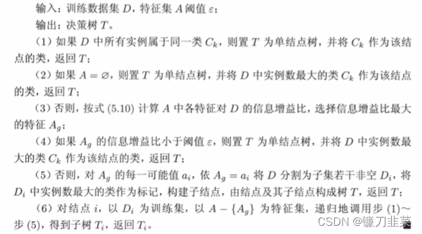

In these two algorithms Control the depth or width of the generated tree by setting a threshold , This practice is called pre pruning . Another way is After generating the decision tree , Then prune , It's called back pruning .

4. Pruning of the decision tree

The decision tree generation algorithm recursively generates the decision tree , Until it can't continue . The tree generated in this way often classifies the training data very accurately , But the classification of unknown test data is not so accurate , That is to say Over fitting phenomenon . The solution to this problem is to consider reducing the complexity of the decision tree , Simplify the generated decision tree .

The process of simplifying the generated tree in decision tree learning is called prune (pruning). Pruning cuts some subtree or leaf nodes from the generated tree , And take its root node or parent node as a new leaf node , So as to simplify the classification tree model .

Decision tree pruning often By minimizing the loss function of the whole decision tree （loss function） To achieve .
Set tree T The number of leaf nodes is |T|,t It's a tree. T Leaf nodes of , The leaf node has $N_t$ A sample points , among k The sample points of class are $N_{tk}$ individual ,$k=1,2,...,K$,$H_t(T)$ For leaf nodes t Empirical entropy on ,$\alpha \ge 0$ Is the parameter , Then the loss function of decision tree learning can be defined as ：
$$C_{\alpha }(T)=\sum _{t=1}^{|T|}{N}_t{H}_t(T)+\alpha |T|$$
Where the empirical entropy is ：
$$H_t(T)=-\sum _k\frac{N_{tk}}{N_t}\log \frac{N_{tk}}{N_t}$$
among ,$C(T)$ Represents the prediction error of the model to the training data , That is, the fitting degree of the model and the training data , When the entropy of leaf nodes is smaller , That is, the smaller the loss , Represents the lower the level of chaos , The better the classification ;

$\mid T\mid$ Represents the complexity of the model . When the number of leaf nodes is larger , It shows that the more complex the decision tree , The worse the generalization ability . The larger $\alpha$ Promote the selection of simpler trees . When $\alpha =0$ It means only considering the fitting degree between the model and the training data , Regardless of complexity .

prune , Is that when $\alpha$ When it's certain , Choose the model with the smallest loss function . The decision tree generation algorithm learns local models , The decision tree pruning learning model as a whole .

Algorithm （ Tree pruning algorithm ）：
Input ： Generate the whole tree of algorithm Chen Sheng T, Parameters $\alpha$
Output ： The sub tree after construction $T_{\alpha }$
（1） Calculate the empirical entropy of each node
（2） Recursively retract from the leaf node of the tree .
（3） If a group of leaf nodes retract to the whole tree before and after the parent node, they are $T_B$ And $T_A$, The corresponding loss functions are $C_{\alpha }(T_B)$ And $C_{\alpha }(T_A)$, if $C_{\alpha }(T_A)\le C_{\alpha }(T_B)$, Then prune , Change the parent node into a new leaf node ;
（4） Return steps 2, Until we can't continue , Get the subtree with the smallest loss function $T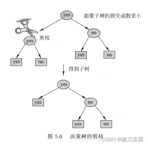_{\alpha }$
Simply speaking , Namely If you subtract a branch , Make this branch a leaf node , The loss function corresponding to the new tree is smaller , Then you can prune , Otherwise, you can't prune .

5. CART Algorithm

Classification and regression trees （classification and regression tree, CART） Model is a widely used decision tree learning method . It can be used for both classification and regression .

The decision tree it generates is a binary tree . It's described above ID3 Algorithm and C4.5 In the algorithm, , If one of the features has more than one ( More than two ) Category , Then it needs to be divided into multiple branches . however CART Algorithm no matter how many categories , It is only divided into two parts .

CART The algorithm consists of the following two steps ：
（1） Decision tree generation ： Generating decision tree based on training data set , The decision tree should be as large as possible ;
（2） Decision tree pruning ： Prune the generated tree with the validation data set and select the optimal subtree , In this case, the minimum loss function is used as the pruning criterion .

5.1 CART Generate

The generation of decision tree is the process of Constructing Binary Decision Tree recursively . Use the square error minimization criterion for the regression tree , Use Gini index for classification tree （Gini index） Minimization criterion , Make feature selection , Generate binary tree .

1. The formation of regression trees

hypothesis X and Y Input and output variables , also Y Is a continuous variable , Given data set $D=\{(x_1,y_1),(x_2,y_2),,...,(x_N,y_N)\}$, Consider how to generate a regression tree .

A regression tree corresponds to the input space （ Feature space ） And the output value on the divided unit . Suppose that the input space has been divided into M A unit $R_1,R_2,...,R_M$, And in each unit $R_m$ It has a fixed output value on it $c_m$, So the regression tree model can be expressed as
$$f(x)=\sum _{m=1}^M{c}_{m}I(x\in R_m)$$
When the partition of the input space is determined , You can use the squared error ${\sum }_{x_i\in R_m}(y_i-f(x_i){)}^2$ To express the prediction error of the regression tree on the training data , The optimal output value of each element is solved by the criterion of minimum square error .

Easy to know , unit $R_m$ Upper $c_m$ The optimal value ${\hat{c}}_m$ yes $R_m$ All input instances on $x_i$ Corresponding output $y_i$ The average of , namely
$${\hat{c}}_m=ave(y_i|x_i\in R_m)$$
The problem is how to divide the input space . Here the heuristic Methods , Select the first j A variable $x^{(j)}$ And the value it takes $s$ As a segmentation variable （spliting variable） And the syncopation point （spliting potting）, And define two regions ：
$$R_1(j,s)=\{x|x^{(j)}\le s\}and{R}_2(j,s)=\{x|x^{(j)}>s\}$$
Then find the optimal segmentation variable j And the optimal tangent point s. In particular , solve
$$\underset{j,s}{\min }[\underset{c_1}{\min }\sum _{x_i\in R_1(j,s)}(y_i-c_1{)}^2+\underset{c_2}{\min }\sum _{x_i\in R_2(j,s)}(y_i-c_2{)}^2]$$
For fixed input variables j You can find the optimal tangent point s.
$${\hat{c}}_1=ave(y_i|x_i\in R_1(j,s))and{\hat{c}}_2=ave(y_i|x_i\in R_2(j,s))$$
Traverse all input variables , Find the optimal segmentation variable j, Form a pair of (j, s). According to this, the input space is divided into two trends . next , Repeat the above division process for each area . Until the stop condition is met , This generates a regression tree . Such a regression tree is usually called Least squares regression tree （least squares regression tree）.
Algorithm （ Least square regression tree generation algorithm ）：
Input ： Training data set D
Output ： Back to the tree $f(x)$
In the input space where the training data set is located , Recursively divide each region into two sub regions and determine the output value on each sub region , Building binary decision tree ;
（1） Choose the best segmentation variable j And the syncopation point s, solve ：
$$\underset{j,s}{\min }[\underset{c_1}{\min }\sum _{x_i\in R_1(j,s)}(y_i-c_1{)}^2+\underset{c_2}{\min }\sum _{x_i\in R_2(j,s)}(y_i-c_2{)}^2]$$
Traverse the variable j, For fixed segmentation variables j Scanning segmentation point s, Select the pair that minimizes the above formula (j, s).
（2） Use the selected right (j, s) Divide the area and determine the output value of the response ：
$$R_1(j,s)=\{x|x^{(j)}\le s\}and{R}_2(j,s)=\{x|x^{(j)}>s\}$$
$${\hat{c}}_m=\frac{1}{N_m}\sum _{x_i\in R_m(j,s)}{y}_i,x\in R_m,m=1,2$$
（3） Continue calling steps on two sub areas （1）（2）. Until the stop condition is met .
（4） Divide the input space into M Regions $R_1,R_2,...,R_M$, Generate decision tree ：
$$f(x)=\sum _{m=1}^M{\hat{c}}_{m}I(x\in R_m)$$

2. The generation of the classification tree
   The classification tree uses Gini index to select the best features , At the same time, the optimal binary segmentation point of the feature is determined .
   Definition （ gini index ） Classification problem . Suppose there is $K$ Classes , The sample point is the first $k$ The probability of each class is $p_k$, Then the gini index of the probability distribution is defined as $$Gini(p)=\sum _{k=1}^K{p}_k(1-p_k)=1-\sum _{k=1}^K{p}_k^2\text{\hspace{1em}(5.12)}$$
   It's used here ${\sum }_{k=1}^K{p}_k=1$
   For class II Classification Problems , If the sample point belongs to the 1 The probability of each class is p, Then the Gini index of the probability distribution is
   $$Gini(p)=2p(1-p)$$
   For a given set of samples D, Its Gini index is
   $$Gini(D)=1-\sum _{k=1}^K(\frac{C_k}{D}{)}^2$$
   here ,$C_k$ yes D Belong to No k Sample subset of class ,K It's the number of classes .

If the sample set D According to the characteristics of A Whether to take a possible value a Be divided into $D_1$ and $D_2$ Two parts , namely
$$D_1=\{(x,y)\in D|A(x)=a\},D_2=D-D_1$$
It's in the characteristics A Under the condition of , aggregate D The Gini index of is defined as
$$Gini(D,A)=\frac{|D_1|}{|D|}Gini(D_1)+\frac{|D_2|}{|D|}Gini(D_2)\text{\hspace{1em}(5.15)}$$
gini index $Gini(D)$ Represents a collection $D$ uncertainty , gini index $Gini(D,A)$ Express the classics $A=a$ Split set $D$ uncertainty . The larger the Gini index , The greater the uncertainty .

The figure below shows the Gini index in the class II classification problem Gini§、 entropy （ Unit bit ） Half $H(p)/2$ And classification error rate . Abscissa represents probability p, The ordinate represents the loss . It can be seen that the curve of Gini index and entropy half is very close , Can approximately represent the classification error rate .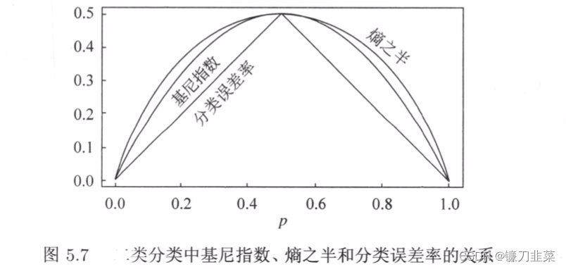

Algorithm （CART generating algorithm ）：
Input ： Training data set D, The conditions for stopping the calculation ;
Output ：CART Decision tree
According to the training data set , Start at the root node , Recursively perform the following operations on each node , Building binary decision tree ：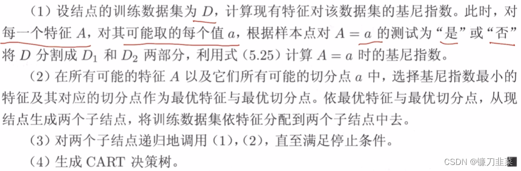

5.2 CART prune

CART Pruning algorithm from ” Complete growth “ Subtract some subtrees from the bottom of the decision tree , Make the decision tree smaller （ The model becomes simpler ）, So that we can have a more accurate prediction of unknown data .
CART The pruning algorithm consists of two steps ： First, the decision tree generated from the generation algorithm $T_0$ The bottom begins to prune constantly , until $T_0$ The root node , Form a sub sequence tree $\{T_0,T_1,...,T_n\}$; And then through Cross validation Test the subtree sequence on an independent validation data set , Select the optimal subtree .

1. prune , Form a sub sequence tree
   In the pruning process , Calculate the loss function of the subtree $$C_{\alpha }(T)=C(T)+\alpha |T|$$, among T For any subtree ,C(T) For the prediction error of training data （ Such as Gini index ）,$|T|$ Is the number of leaf nodes of the subtree ,$\alpha \ge 0$ Is the parameter ,$C_{\alpha }(T)$ The parameter is $\alpha$ Time subtree T The overall loss of . Parameters $\alpha$ Weigh the fitting degree of training data and the complexity of the model .
   To be fixed $\alpha$, There must be a loss function $C_{\alpha }(T)$ The smallest subtree , Express it as $T_{\alpha }$.$T_{\alpha }$ In loss function $C_{\alpha }(T)$ It is optimal in the smallest sense .

2. The subtree sequence obtained by pruning $\{T_0,T_1,...,T_n\}$ The optimal subtree is selected through cross validation $T_{\alpha }$
   In particular , Using independent validation data sets , Test subtree sequence $T_0,T_1,...,T_n$ Square error or Gini index of each tree in . The decision tree with the smallest square error or Gini index is considered to be the optimal decision tree . In the subtree sequence , Each subtree $T_0,T_1,...,T_n$ All correspond to a parameter ${\alpha }_1,{\alpha }_2,...{\alpha }_n$, therefore , When the optimal subtree $T_k$ When it's certain , Corresponding ${\alpha }_k$ It's also certain that , That is, the optimal decision tree $T_{\alpha }$.
   Algorithm （CART Pruning algorithm ）
   Input ：CART Algorithm generated decision tree $T_0$
   Output ： Optimal decision tree $T_{\alpha }$
   （1） set up $k=0,T=T_0$
   （2） set up $\alpha =+\infty$
   （3） From bottom to top to each internal node t Calculation $C(T)$,$|T_t|$ as well as $g(t)=\frac{C(t)-C(T_t)}{|T_t-1|},\alpha =\min (\alpha ,g(t))$, here ,$T_t$ Said to t The subtree of the root node ,$C(T_t)$ It's the prediction error of training data ,$|T_t|$ yes $T_t$ The number of leaf nodes of .
   （4） Yes $g(t)=\alpha$ Internal node of t Pruning , And for leaf nodes t With Majority voting Determine its class , Get the tree T
   （5） set up $k=k+1,{\alpha }_k=\alpha ,T_k=T$
   （6） If $T_k$ It is not a tree composed of root node and two leaf nodes , Then go back to step （3）; Otherwise the $T_k=T_n$
   （7） Using cross validation in subtree sequence $\{T_0,T_1,...,T_n\}$ Select the best subtree $T_{\alpha }$.

summary

No matter what ID3,C4.5,CART It is to choose an optimal feature to make classification decision , But most , Classification decision is not determined by a certain feature , It's a set of features . The decision tree obtained in this way is more accurate , This decision tree is called Multivariate decision trees (multi-variate decision tree). When selecting the best feature , Multivariable decision tree is not to select an optimal feature , Instead, choose an optimal linear combination of features to make a decision . Representative algorithm OC1.

Advantages of decision trees ：
（1） Compared to black box classification models like neural networks , The decision tree can be explained logically .
（2） You can deal with both discrete and continuous values . Many algorithms just focus on discrete or continuous values .
（3） The cost of using decision tree prediction is O(log2m).m Sample size .
（4） Good fault tolerance for outliers , High robustness .

Disadvantages of using decision trees ：
（1） Decision tree algorithm is very easy to over fit , This leads to weak generalization ability . It can be improved by setting the minimum number of samples and limiting the depth of decision tree .
（2） The decision tree will change a little because of the sample , Cause dramatic changes in tree structure . This can be solved by integrated learning and so on .
（3） If the sample size of some features is too large , Generating decision trees tends to favor these features . This can be improved by adjusting the sample weight .

Reference material

[1] 《 Statistical learning method 》 expericnce
[2] You know ： Little 《 Statistical learning method 》（ The fifth chapter ） Decision tree