当前位置:网站首页>4. Cross entropy
4. Cross entropy
2022-07-08 01:02:00 【booze-J】
article
Cross entropy (cross-entropy)
1. Quadratic cost function (quadratic cost)
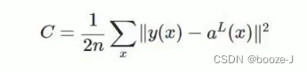
among ,c It's a cost function ,x Presentation sample ,y Represents the actual value ,a Represents the output value ,n Represents the total number of samples . For the sake of simplicity , Use a sample as an example to illustrate , At this time, the quadratic cost function is :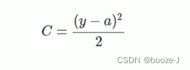
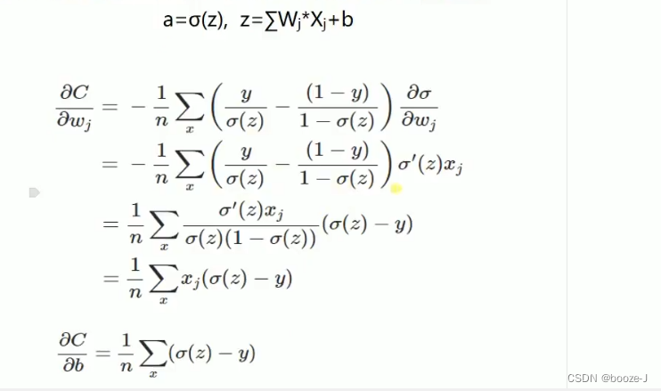
Suppose we use the gradient descent method (Gradient descent) To adjust the size of the weight parameter , A weight w And offset b The gradient of is derived as follows :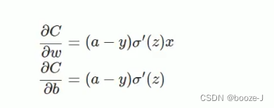
among ,z Represents the input of a neuron , α \alpha α Is the activation function .w and b Is proportional to the gradient of the activation function , The greater the gradient of the activation function ,w and b The faster you resize , The faster the training converges . Suppose our activation function is sigmoid function :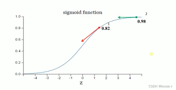
Suppose our goal is to converge to 1.0.1 Points for 0.82 It's far from the target , The gradient is bigger , The weight adjustment is relatively large .2 Points for 0.98 Closer to the target , The gradient is smaller , The weight adjustment is relatively small . The adjustment plan is reasonable .
If our goal is to converge to 0.1 Points for 0.82 The goal is relatively close , The gradient is bigger , The weight adjustment is relatively large .2 Points for 0.98 It's far from the target , The gradient is smaller , The weight adjustment is relatively small . The adjustment plan is unreasonable .
2. Cross entropy cost function (cross-entropy)
Another way of thinking , We don't change the activation function , It's changing the cost function , Use the cross entropy cost function instead :
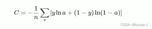
among ,C It's a cost function ,x Presentation sample ,y Represents the actual value ,a Represents the output value ,n Represents the total number of samples .
If the output neuron is linear , Then the quadratic cost function is a suitable choice . If the output neuron is S Type of function , Then it is more suitable to use the cross entropy cost function .
3. Logarithmic interpretive cost function (log-likelihood cost)
Logarithmic interpretive function is often used as softmax The cost function of regression , Then the neurons in the output layer are sigmoid function , Cross entropy cost function can be used . The more common practice in deep learning is to softmax As the last layer , At this time, the commonly used cost function is the logarithmic interpretive cost function .
Log likelihood cost function and softmax The combination and cross entropy of sigmoid The combination of functions is very similar . Logarithmic interpretive cost function can be reduced to the form of cross drop cost function in binary classification .
stay tensorflow of use :tf.nn.sigmoid_cross_entropy_with_logits() To show the following sigmoid Cross line for collocation .tf.nn.softmax_cross_entropy with_logits() To show the following softmax Cross line for collocation .
Easy to use
We apply it to 3.MNIST Data set classification In the code in , Just modify a simple sentence .
take 3. In the training model
#  Define optimizer ,loss_function, The accuracy of calculation during training
model.compile(
    optimizer=sgd,
    loss="mse",
    metrics=['accuracy']
)
It is amended as follows
#  Define optimizer ,loss_function, The accuracy of calculation during training
model.compile(
    optimizer=sgd,
    loss="categorical_crossentropy",
    metrics=['accuracy']
)
Then run the whole code :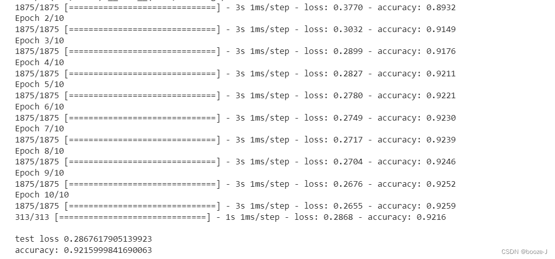
contrast 3.MNIST Data set classification Results of operation , It can be found that the classification model using cross entropy as the loss function can make the model converge faster , The effect is better. .
Complete code
The code running platform is jupyter-notebook, Code blocks in the article , According to jupyter-notebook Written in the order of division in , Run article code , Glue directly into jupyter-notebook that will do .
1. Import third-party library
import numpy as np
from keras.datasets import mnist
from keras.utils import np_utils
from keras.models import Sequential
from keras.layers import Dense
from tensorflow.keras.optimizers import SGD
2. Loading data and data preprocessing
#  Load data
(x_train,y_train),(x_test,y_test) = mnist.load_data()
# (60000, 28, 28)
print("x_shape:\n",x_train.shape)
# (60000,)  Not yet one-hot code   You need to operate by yourself later
print("y_shape:\n",y_train.shape)
# (60000, 28, 28) -> (60000,784) reshape() Middle parameter filling -1 Parameter results can be calculated automatically   Divide 255.0 To normalize
x_train = x_train.reshape(x_train.shape[0],-1)/255.0
x_test = x_test.reshape(x_test.shape[0],-1)/255.0
#  in one hot Format
y_train = np_utils.to_categorical(y_train,num_classes=10)
y_test = np_utils.to_categorical(y_test,num_classes=10)
3. Training models
#  Creating models   Input 784 Neurons , Output 10 Neurons
model = Sequential([
        #  Define output yes 10  Input is 784, Set offset to 1, add to softmax Activation function
        Dense(units=10,input_dim=784,bias_initializer='one',activation="softmax"),
])
#  Define optimizer
sgd = SGD(lr=0.2)

#  Define optimizer ,loss_function, The accuracy of calculation during training
model.compile(
    optimizer=sgd,
    loss="categorical_crossentropy",
    metrics=['accuracy']
)
#  Training models
model.fit(x_train,y_train,batch_size=32,epochs=10)

#  Evaluation model
loss,accuracy = model.evaluate(x_test,y_test)

print("\ntest loss",loss)
print("accuracy:",accuracy)
边栏推荐
- 大二级分类产品页权重低,不收录怎么办?
- Introduction to ML regression analysis of AI zhetianchuan
- ThinkPHP kernel work order system source code commercial open source version multi user + multi customer service + SMS + email notification
- NVIDIA Jetson test installation yolox process record
- 基于微信小程序开发的我最在行的小游戏
- Analysis of 8 classic C language pointer written test questions
- 国内首次,3位清华姚班本科生斩获STOC最佳学生论文奖
- New library online | information data of Chinese journalists
- Basic mode of service mesh
- C#中string用法
猜你喜欢
Interface test advanced interface script use - apipost (pre / post execution script)
Malware detection method based on convolutional neural network
8道经典C语言指针笔试题解析
Complete model verification (test, demo) routine
Cancel the down arrow of the default style of select and set the default word of select
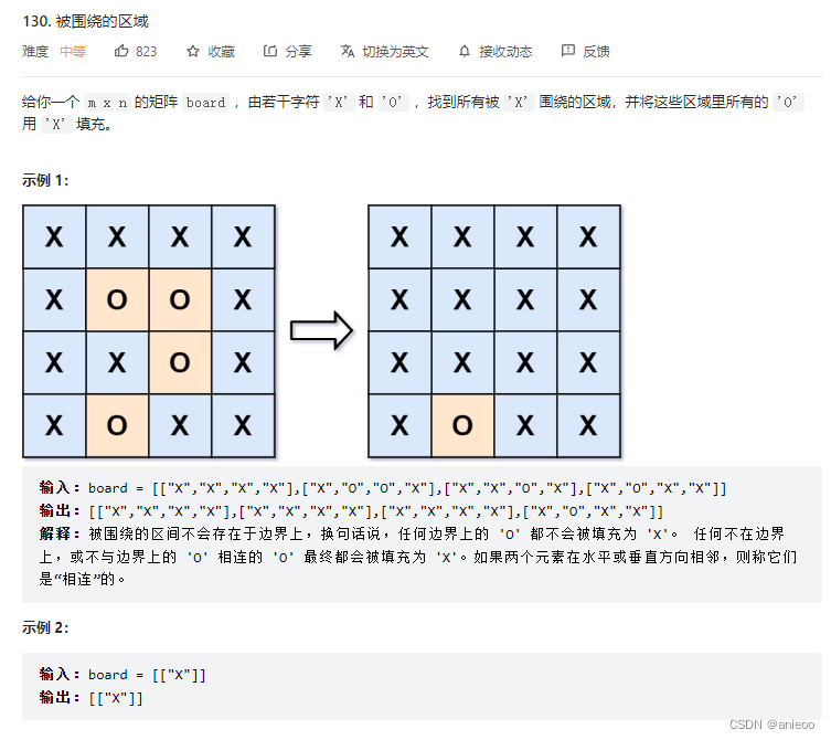
130. 被圍繞的區域
Y59. Chapter III kubernetes from entry to proficiency - continuous integration and deployment (III, II)
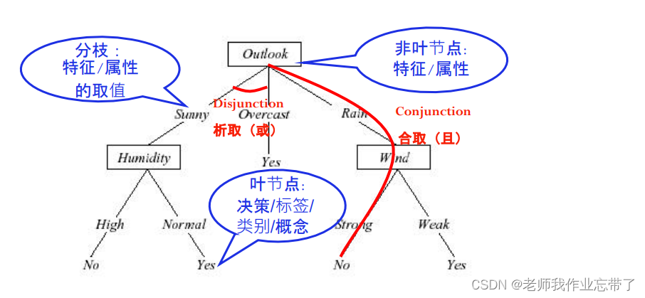
AI遮天传 ML-初识决策树
新库上线 | CnOpenData中华老字号企业名录
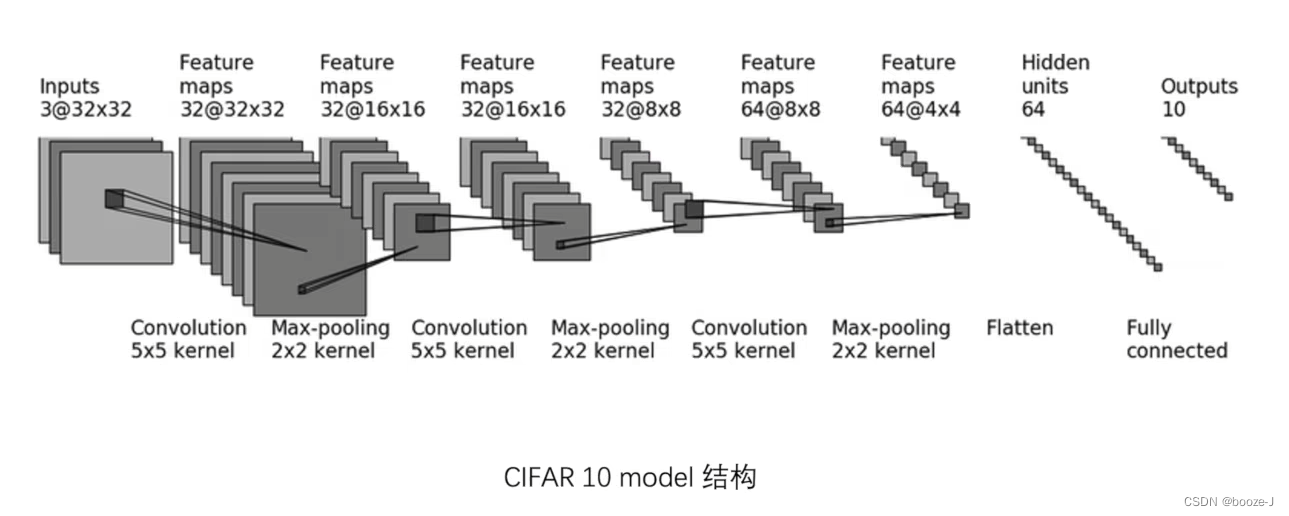
9. Introduction to convolutional neural network
随机推荐
Invalid V-for traversal element style
C # generics and performance comparison
They gathered at the 2022 ecug con just for "China's technological power"
Prediction of the victory or defeat of the League of heroes -- simple KFC Colonel
基于卷积神经网络的恶意软件检测方法
13.模型的保存和載入
[Yugong series] go teaching course 006 in July 2022 - automatic derivation of types and input and output
Analysis of 8 classic C language pointer written test questions
[Yugong series] go teaching course 006 in July 2022 - automatic derivation of types and input and output
y59.第三章 Kubernetes从入门到精通 -- 持续集成与部署(三二)
Letcode43: string multiplication
丸子官网小程序配置教程来了(附详细步骤)
C# ?,?.,?? .....
13. Enregistrement et chargement des modèles
牛客基础语法必刷100题之基本类型
《因果性Causality》教程,哥本哈根大学Jonas Peters讲授
网络模型的保存与读取
国外众测之密码找回漏洞
手机上炒股安全么?
【obs】Impossible to find entrance point CreateDirect3D11DeviceFromDXGIDevice