当前位置:网站首页>Chapter IV decision tree
Chapter IV decision tree
2022-07-08 01:07:00 【Intelligent control and optimization decision Laboratory of Cen】
Which parts does the decision tree learning algorithm include ? What are the commonly used algorithms ?
The learning algorithm of decision tree mainly includes three parts :
1. feature selection 2. The generation of trees 3. Pruning of trees
There are several commonly used algorithms :
1.ID3 2. C4.5 3.CART
Root node of decision tree 、 What do internal nodes and leaf nodes represent respectively ?
The leaf node corresponds to the decision result , Each other node corresponds to an attribute test ; The sample set contained in each node is divided into sub nodes according to the result of attribute test ; The root node contains the complete set of samples . The path from the root node to each leaf node corresponds to a decision test sequence .
What are the criteria for feature selection ( How to choose the best partition attribute )?
Feature selection is mainly based on information gain and information gain ratio
Information gain
First, the definition of information entropy is : E n t ( D ) = − ∑ k = 1 ∣ y ∣ p k Ent(D)=-\sum_{k=1}^{|y|}p_k Ent(D)=−∑k=1∣y∣pk l o g 2 p k log_2p_k log2pk
The information gain is : G a i n ( D , a ) = E n t ( D ) − ∑ v = 1 V ∣ D v ∣ ∣ D ∣ E n t ( D v ) Gain(D,a)=Ent(D)-\sum_{v=1}^{V}\frac{|D^v|}{|D|}Ent(D^v) Gain(D,a)=Ent(D)−∑v=1V∣D∣∣Dv∣Ent(Dv)
Information gain ratio
The gain ratio is defined as : G a i n Gain Gain_ r a t i o ( D , a ) = G a i n ( D , a ) I V ( a ) , ratio(D,a)=\frac{Gain(D,a)}{IV(a)}, ratio(D,a)=IV(a)Gain(D,a),
among : I V ( a ) = − ∑ v = 1 V ∣ D v ∣ ∣ D ∣ l o g 2 ∣ D v ∣ ∣ D ∣ IV(a)=-\sum_{v=1}^{V}\frac{|D^v|}{|D|}log_2\frac{|D^v|}{|D|} IV(a)=−∑v=1V∣D∣∣Dv∣log2∣D∣∣Dv∣
How to prevent overfitting in decision trees ?
Pruning is a decision tree learning algorithm “ An important means of over fitting ”. In order to prevent the decision tree from learning the training samples too well , The risk of over fitting can be reduced by actively removing some branches . The basic strategies of pruning mainly include “ pre-pruning ” and “ After pruning ”
pre-pruning
It refers to the generation process of decision tree , Estimate each node before partitioning , If the current node partition cannot improve the generalization performance of decision tree , Then the partition is stopped and the current node is marked as a leaf node .
After pruning
After pruning, a complete decision tree is generated from the training set , Then the non leaf nodes are examined from bottom to top , If the subtree corresponding to this node is replaced by leaf nodes, the generalization ability of the decision tree can be improved , Replace the subtree with a leaf node .
How to deal with continuous values and missing values ?
1. Continuous value processing
Because the number of values of continuous attributes is no longer limited , therefore , It is impossible to divide nodes directly according to the values of continuous attributes . here , Discretization technology can be used continuously . The simplest strategy is to use dichotomy to deal with continuous attributes , That's exactly what it is. C4.5 The mechanism used in the decision tree algorithm .
2. Missing value processing
Incomplete samples are often encountered in real tasks , That is, some attribute values of the sample are missing . For example, due to the cost of diagnosis and testing 、 Privacy protection and other factors , The value of some attributes of the patient's medical data ( Such as HIV test result ) Unknown ; Especially when the number of attributes is large , There are often a large number of samples with missing values . If you simply give up incomplete samples , Only samples without missing values can be used for learning , Obviously, it is a great waste of data information .
1. So how to choose the partition attribute when the attribute value is missing ?
ρ \rho ρ Indicates the proportion of samples without missing values , Given training set D D D And attribute a a a, D ^ \hat{D} D^ Express D D D In attributes a a a Sample subset with no missing values on .
G a i n ( D , a ) = ρ ∗ G a i n ( D ^ , a ) Gain(D,a)=\rho*Gain(\hat{D},a) Gain(D,a)=ρ∗Gain(D^,a)
2. Given partition properties , If the value of the sample on the attribute is missing , How to divide the samples ?
If sample x x x In dividing attributes a a a The value on is known , Will x x x Transfer in the child node corresponding to its value , And the sample weight is maintained as w x w_x wx; If sample X X X In dividing attributes a a a Unknown value on , Will X X X Transfer in all child nodes at the same time , And the sample weight lies in the attribute value a v a^v av The corresponding sub nodes are adjusted to r ^ v ∗ w x \hat{r}_v*{w_x} r^v∗wx, among r ^ v \hat{r}_v r^v Indicates the attribute in the sample without missing value a a a Top value a v a^v av The proportion of the sample of .
边栏推荐
猜你喜欢
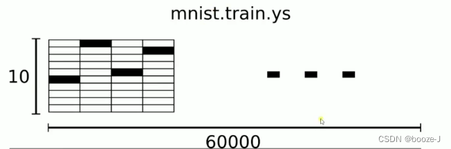
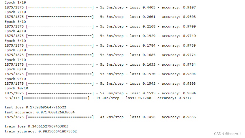
3.MNIST数据集分类
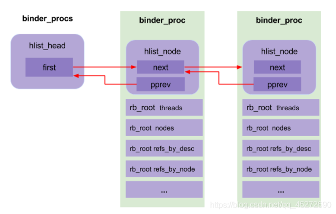
Binder core API
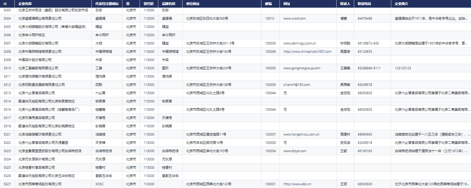
New library launched | cnopendata China Time-honored enterprise directory
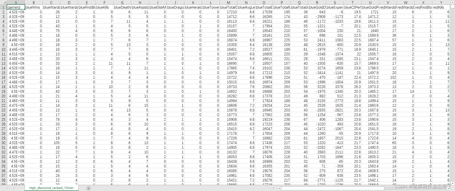
英雄联盟胜负预测--简易肯德基上校
国外众测之密码找回漏洞
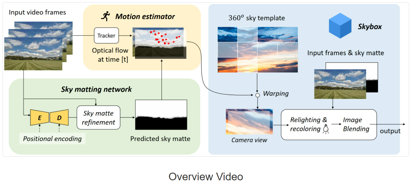
【深度学习】AI一键换天

Cancel the down arrow of the default style of select and set the default word of select
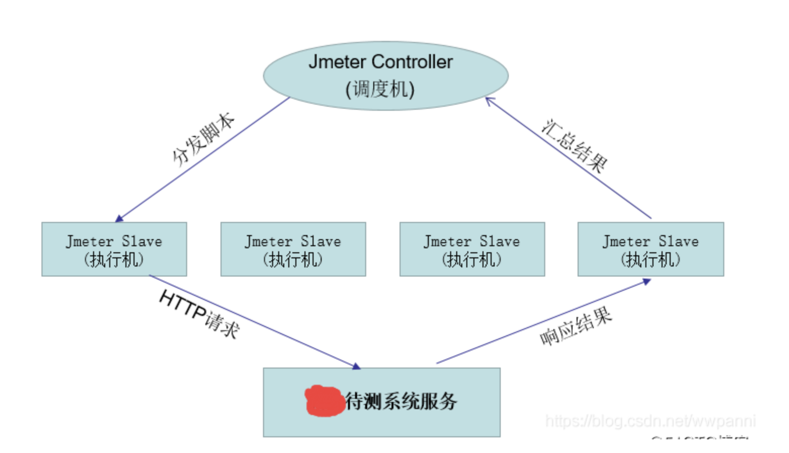
jemter分布式
7.正则化应用
![[Yugong series] go teaching course 006 in July 2022 - automatic derivation of types and input and output](/img/79/f5cffe62d5d1e4a69b6143aef561d9.png)
[Yugong series] go teaching course 006 in July 2022 - automatic derivation of types and input and output
随机推荐
Hotel
German prime minister says Ukraine will not receive "NATO style" security guarantee
SDNU_ACM_ICPC_2022_Summer_Practice(1~2)
Is it safe to speculate in stocks on mobile phones?
How to use education discounts to open Apple Music members for 5 yuan / month and realize member sharing
50Mhz产生时间
DNS series (I): why does the updated DNS record not take effect?
swift获取url参数
Su embedded training - Day5
11.递归神经网络RNN
Interface test advanced interface script use - apipost (pre / post execution script)
大二级分类产品页权重低,不收录怎么办?
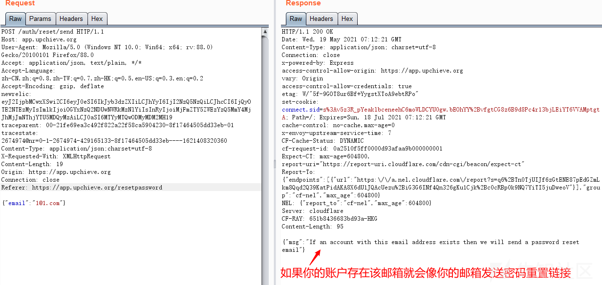
Password recovery vulnerability of foreign public testing
2.非线性回归
基于人脸识别实现课堂抬头率检测
130. 被围绕的区域
Kubernetes static pod (static POD)
Service Mesh的基本模式
Share a latex online editor | with latex common templates
Codeforces Round #804 (Div. 2)(A~D)