当前位置:网站首页>Practical cases, hand-in-hand teaching you to build e-commerce user portraits | with code
Practical cases, hand-in-hand teaching you to build e-commerce user portraits | with code
2022-07-06 14:57:00 【Python advanced】
Click on the above “Python Crawler and data mining ”, Focus on
reply “ Books ” You can get a gift Python From the beginning to the advanced stage 10 This ebook
today
Japan
chicken
soup
I want to take a branch of the river and sea , A visit to Zhaoling .
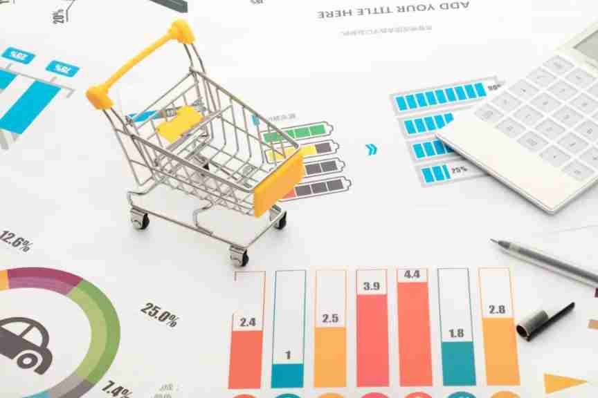
Reading guide : This paper takes a real case , Teach you to build user portraits of e-commerce systems hand in hand .
Let's first look at the labels used in the e-commerce user portrait .
Data content includes user_id( User's identity )、item_id( goods )、IDbehavior_type( User behavior type , Include click 、 Collection 、 Plus shopping cart 、 There are four ways to pay , Separate numbers 1、2、3、4 Express )、user_geohash( Location )、item_category( category ID, That is, the category to which the commodity belongs )、Time( When does the user behavior occur ), among user_id and item_id Because it's about privacy , Desensitized , It shows the number .
The following is the specific code implementation process .
01
Import library
In addition to numpy、pandas、matplotlib, Other modules are also used .
1#  Import the required Library
 2
 3%matplotlib inline
 4
 5import numpy as np
 6
 7import pandas as pd
 8
 9from matplotlib import pyplot as plt
10
11from datetime import datetime
The parameters are described as follows .
%matplotlib inline: A magic function , because %matplotlib inline The existence of , When the input plt.plot() after , There is no need to enter plt.show(), The image will be displayed automatically .
datetime: Module used to display time .
02
Data preparation
1#  Import dataset
2
3df_orginal = pd.read_csv('./taobao_persona.csv')
4
5#  Extract some data
6
7df = df_orginal.sample(frac=0.2,random_state=None)
Use here Pandas Of read_csv Method to read the data file , Because the data set is too large , In order to improve operation efficiency , Use sample Function random extraction 20% The data of .
DataFrame.sample() yes Pandas The function in ,DataFrame Is a data format , Generation refers to df_orginal.frac(fraction) Is how much data to extract ,random_state It's a random number seed , The purpose is to ensure that the data randomly selected each time is the same , Prevent using different data when executing commands .
03
Data preprocessing
1#  Check whether there are missing values , Count the missing values of each field
 2
 3df.isnull().any().sum()
 4
 5#  Only found user_geohash Missing values , And the proportion of missing is very high , There is no significance of statistical analysis , Delete this column
 6
 7df.drop('user_geohash',axis=1,inplace=True)
 8
 9#  take time The field is split into date and period
10
11df['date'] = df['time'].str[0:10]
12
13df['time'] = df['time'].str[11:]
14
15df['time'] = df['time'].astype(int)
16
17# date use str Method access 0-9 A character ,time take 11 To the last , take time Turn it into int type .
18
19#  Divide the period into ' In the morning ',' In the morning ',' At noon, ',' Afternoon ',' evening '
20
21df['hour'] = pd.cut(df['time'],bins=[-1,5,10,13,18,24],labels=[' In the morning ',' In the morning ',
22
23    ' At noon, ',' Afternoon ',' evening '])
The result is shown in Fig. 1 Shown .
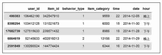
chart 1 Data preprocessing results
1#  Generate user label table , All the labels made are added to this table
2
3users = df['user_id'].unique()
4
5labels = pd.DataFrame(users,columns=['user_id'])
pd.DataFrame(): The data is filled with users, Column name is user_id.
The result is shown in Fig. 2 Shown .
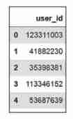
chart 2 Produced users ID
After that, the analyzed content will be placed in this table , It is equivalent to establishing a blank table , Add the conclusions of your analysis one by one .
04
Number of build user behavior tags
1) Analyze user browsing time period
Select the time period that each user browses the most , See when users browse more products .
1#  Group users and time periods , Count the number of views
 2
 3time_browse = df[df['behavior_type']==1].groupby(['user_id','hour']).item_
 4
 5    id.count().reset_index()
 6
 7time_browse.rename(columns={'item_id':'hour_counts'},inplace=True)
 8
 9#  Count the time period that each user browses the most
10
11time_browse_max = time_browse.groupby('user_id').hour_counts.max().reset_index()
12
13time_browse_max.rename(columns={'hour_counts':'read_counts_max'},inplace=True)
14
15time_browse = pd.merge(time_browse,time_browse_max,how='left',on='user_id')
16
17#  Previously, according to user_id and hour Count and count the times of browsing items , Now borrow the statistics of browsing times user_id stay
18
19#  Which time period has the most views , And take it as the representative of the user's browsing time tag .
20
21#  Select the time period with the most views of each user , If there is the most tied period , Connect... With commas
22
23time_browse_hour=time_browse.loc[time_browse['hour_counts']==time_browse['read_
24
25    counts_max'],'hour'].groupby(time_browse['user_id']).aggregate(lambda
26
27    x:','.join(x)).reset_index()
28
29time_browse_hour.head()
30
31#  Add the active period of user browsing to the user tag table
32
33labels = pd.merge(labels,time_browse_hour,how='left',on='user_id')
34
35labels.rename(columns={'hour':'time_browse'},inplace=True)
36
37# labels Equivalent to an examination paper , The above shows the final results
The result is shown in Fig. 3 Shown .
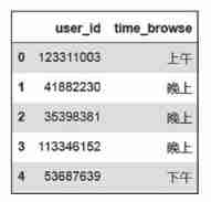
chart 3 User browsing period
groupby(['key1','key2']): Multi column aggregation , The grouping key is column name .
reset_index(): Default drop=False, You can get new index, The original index Become a data column and keep it , The first column will add the number of counts , Will not use index.
rename(): Rename , Here will be item_id Replace with hour_counts,inplace Whether to fill in place .
pd.merge(): Merge the two tables together , Horizontal merger ,on Represents a primary key ,how Left pointing merge , Each line corresponds one by one .
loc function : By row index Index To get the specified data .
aggregate function :groupby After grouping, multiple sub data frames will be returned , This function can realize data aggregation , You can get some information of some columns of each sub data frame .
lambda function : You can define an anonymous function ,lambda [arg1[, arg2, … argN]]: expression, Where the parameter is the input of the function , It's optional , The following expression is output , Here and join() Functions together , Each of them x Value can be “,” separate ; Using similar code, you can generate browsing active periods , I won't go into details here .
2) About user behavior of categories .
1df_browse = df.loc[df['behavior_type']==1,['user_id','item_id','item_category']]
2
3df_collect = df.loc[df['behavior_type']==2,['user_id','item_id','item_category']]
4
5df_cart = df.loc[df['behavior_type']==3,['user_id','item_id','item_category']]
6
7df_buy = df.loc[df['behavior_type']==4,['user_id','item_id','item_category']]
According to different user behavior , Such as browsing 、 Collection, etc. , Export data separately for analysis .
1#  Group users and categories , Count the number of views
 2
 3df_cate_most_browse = df_browse.groupby(['user_id','item_category']).item_id.count().
 4
 5    reset_index()
 6
 7df_cate_most_browse.rename(columns={'item_id':'item_category_counts'},inplace=
 8
 9    True)
10
11#  Count the categories that each user browses the most
12
13df_cate_most_browse_max=df_cate_most_browse.groupby('user_id').item_category_
14
15    counts.max().reset_index()
16
17df_cate_most_browse_max.rename(columns={'item_category_counts':'item_category_
18
19    counts_max'},inplace=True)
20
21df_cate_most_browse = pd.merge(df_cate_most_browse,df_cate_most_browse_max,
22
23    how='left',on='user_id')
24
25#  take item_category The number type of is changed to string
26
27df_cate_most_browse['item_category'] = df_cate_most_browse['item_category'].
28
29    astype(str)
30
31#  Select the category with the most views by each user , If there is a category with the most juxtaposition , Connect... With commas
32
33df_cate_browse=df_cate_most_browse.loc[df_cate_most_browse['item_category_
34
35    counts']==
36
37df_cate_most_browse['item_category_counts_max'],'item_category'].groupby(df_
38
39    cate_most_browse['user_id']).aggregate(lambda x:','.join(x)).reset_index()
40
41#  Add the most browsed categories to the user tab
42
43labels = pd.merge(labels,df_cate_browse,how='left',on='user_id')
44
45labels.rename(columns={'item_category':'cate_most_browse'},inplace=True)
46
47labels.head(5)
The categories that users browse most are shown in the figure 4 Shown .
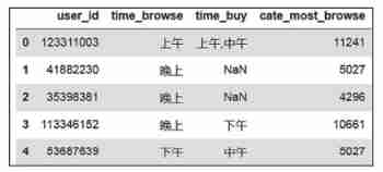
chart 4 The most viewed categories
Collection 、 The generation logic of the category with the most additional purchases and purchases is the same , The results after repeated operation are shown in the figure 5 Shown .
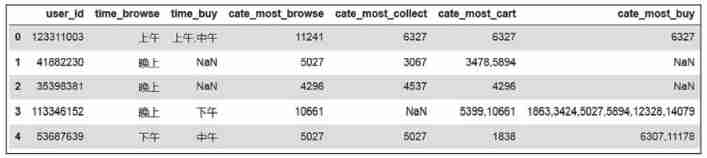
chart 5 About user behavior of categories
We can see from the data , Browse 、 Plus shopping cart 、 Collection 、 In fact, there is not necessarily an obvious inevitable relationship before buying , We need further analysis to get some rules .
3) near 30 Day user behavior analysis .
near 30 Number of purchases per day :
1#  Group purchasing behaviors by users , Count the times
2
3df_counts_30_buy = df[df['behavior_type']==4].groupby('user_id').item_id.
4
5    count().reset_index()
6
7labels = pd.merge(labels,df_counts_30_buy,how='left',on='user_id')
8
9labels.rename(columns={'item_id':'counts_30_buy'},inplace=True)
near 30 Number of additional purchases per day :
1#  Group additional purchases by users , Count the times
2
3df_counts_30_cart = df[df['behavior_type']==3].groupby('user_id').item_id.
4
5    count().reset_index()
6
7labels = pd.merge(labels,df_counts_30_cart,how='left',on='user_id')
8
9labels.rename(columns={'item_id':'counts_30_cart'},inplace=True)
near 30 Days active days :
1#  Group users , Count the number of active days , Including browsing 、 Collection 、 purchased 、 Buy
2
3counts_30_active = df.groupby('user_id')['date'].nunique()
4
5labels = pd.merge(labels,counts_30_active,how='left',on='user_id')
6
7labels.rename(columns={'date':'counts_30_active'},inplace=True)
8
9 here pd.nunique() It refers to the number of unique values returned .
The result is shown in Fig. 6 Shown .
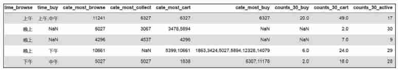
chart 6 near 30 Day user behavior
near 30 Day user behavior analysis belongs to medium and long-term user behavior , We can judge whether we need to adjust the marketing strategy , Similar can get short-term 7 Day user behavior analysis , Observe the medium and short term or a small cycle , What is the behavior of users .
4) Days since the last behavior .
Analyzing the time difference between the last time and this time can achieve accurate recommendation analysis , Now let's see how to realize .
Days since last browse :
1days_browse = df[df['behavior_type']==1].groupby('user_id')['date'].max().apply
2
3(lambda x:(datetime.strptime('2014-12-19','%Y-%m-%d')-x).days)
4
5labels = pd.merge(labels,days_browse,how='left',on='user_id')
6
7labels.rename(columns={'date':'days_browse'},inplace=True)
datetime.strptime('2014-12-19','%Y-%m-%d')-x).days: This part belongs to lambda Function expression part in , Calculation rules , Here, the sum of days after subtraction is finally taken .
apply(): The format is apply(func,*args,**kwargs), When the parameters of a function exist in a tuple or a dictionary , This function can be called indirectly , And pass the parameters in tuples or dictionaries to the function in order , The return value is func The return value of the function . Equivalent to loop traversal , Play the effect of processing every piece of data .
Similar to the last additional purchase 、 Days since purchase , Analyze the activity of users , Pictured 7 Shown , If you haven't been active for a long time , You need to push some content , Or issue coupons to stimulate users .
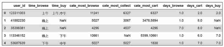
chart 7 Statistics of the last behavior from today
5) The number of days between the last two purchases .
1df_interval_buy = df[df['behavior_type']==4].groupby(['user_id','date']).item_
 2
 3    id.count().reset_index()
 4
 5interval_buy = df_interval_buy.groupby('user_id')['date'].apply
 6
 7(lambda x:x.sort_values().diff(1).dropna().head(1)).reset_index()
 8
 9interval_buy['date'] = interval_buy['date'].apply(lambda x : x.days)
10
11interval_buy.drop('level_1',axis=1,inplace=True)
12
13interval_buy.rename(columns={'date':'interval_buy'},inplace=True)
14
15labels = pd.merge(labels,interval_buy,how='left',on='user_id')
Analyze the purchase frequency of users with the number of purchase intervals , It is convenient to determine the consumption activity level of users , Accurately formulate marketing methods . The result is shown in Fig. 8 Shown .
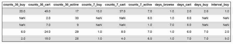
chart 8 Statistics of the number of days between the last two purchases
6) Whether to browse without placing an order .
1df_browse_buy=df.loc[(df['behavior_type']==1)|(df['behavior_type']==4),
 2
 3['user_id','item_id','behavior_type','time']]
 4
 5browse_not_buy=pd.pivot_table(df_browse_buy,index=['user_id','item_id'],
 6
 7columns=['behavior_type'],values=['time'],aggfunc=['count'])
 8
 9browse_not_buy.columns = ['browse','buy']
10
11browse_not_buy.fillna(0,inplace=True)
12
13#  Added a column browse_not_buy, The initial value is 0.
14
15browse_not_buy['browse_not_buy'] = 0
16
17#  Browse the number >0, Number of purchases =0 Data output of 1.
18
19browse_not_buy.loc[(browse_not_buy['browse']>0) & (browse_not_buy['buy']==0),
20
21    'browse_not_buy'] = 1
22
23browse_not_buy=browse_not_buy.groupby('user_id')['browse_not_buy'].sum().reset_
24
25    index()
26
27labels = pd.merge(labels,browse_not_buy,how='left',on='user_id')
28
29labels['browse_not_buy'] = labels['browse_not_buy'].apply(lambda x: ' yes ' if x>0
30
31    else ' no ')
|: stay Python In the statement, it means or ,& To express and .
pd.pivot_table(): Pivot table function ,df_browse_buy by data block ,values You can filter the required calculation data ,aggfunc Parameters can be used to set the function operation when we aggregate data .
fillna: Will fill in NaN data , Returns the filled result ,inplace=True Represents filling in place .
The result is shown in Fig. 9 Shown .
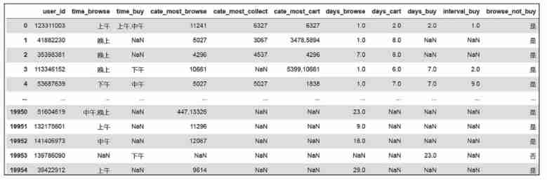
chart 9 Whether to browse the statistics of not placing an order
For users who browse without placing an order, we should strengthen the promotion , You can increase the number of coupons , Promote shopping .
7) Whether additional purchase has not been placed .
1df_cart_buy=df.loc[(df['behavior_type']==3)|(df['behavior_type']==4),['user_
 2
 3    id','item_id','behavior_type','time']]
 4
 5cart_not_buy=pd.pivot_table(df_cart_buy,index=['user_id','item_id'],columns=
 6
 7    ['behavior_type'],values=['time'],aggfunc=['count'])
 8
 9cart_not_buy.columns = ['cart','buy']
10
11cart_not_buy.fillna(0,inplace=True)
12
13cart_not_buy['cart_not_buy'] = 0
14
15cart_not_buy.loc[(cart_not_buy['cart']>0) & (cart_not_buy['buy']==0),'cart_not_
16
17    buy'] = 1
18
19cart_not_buy = cart_not_buy.groupby('user_id')['cart_not_buy'].sum().reset_index()
20
21labels = pd.merge(labels,cart_not_buy,how='left',on='user_id')
22
23labels['cart_not_buy'] = labels['cart_not_buy'].apply(lambda x: ' yes ' if x>0
24
25    else ' no ')
The result is shown in Fig. 10 Shown .
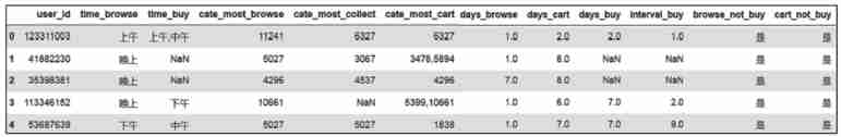
chart 10 Statistics of whether additional purchase has not been placed
When formulating marketing strategies , Pay special attention to this part of the population , Because the purchase conversion rate of additional purchase without order is the largest , There is a successful order 、 The most potential customers are here .
05
Build user attribute tags
1) Whether to re purchase users :
1buy_again = df[df['behavior_type']==4].groupby('user_id')['item_id'].count().
 2
 3    reset_index()
 4
 5buy_again.rename(columns={'item_id':'buy_again'},inplace=True)
 6
 7labels = pd.merge(labels,buy_again,how='left',on='user_id')
 8
 9labels['buy_again'].fillna(-1,inplace=True)
10
11#  Users who have not purchased are marked as ' Not purchased ', Users who have purchased but not re purchased are marked ' no ', Users with re purchase are marked as ' yes '
12
13labels['buy_again'] = labels['buy_again'].apply(lambda x: ' yes ' if x>1 else
14
15    ' no ' if x==1 else ' Not purchased ')
The result is shown in Fig. 11 Shown .
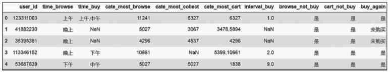
chart 11 Whether to re purchase user statistics
2) Visit activity :
1user_active_level = labels['counts_30_active'].value_counts().sort_index(ascending=
 2
 3    False)
 4
 5plt.figure(figsize=(16,9))
 6
 7user_active_level.plot(title='30 The relationship between the number of visits in a day and the number of visitors ',fontsize=18)
 8
 9plt.ylabel(' Number of visitors ',fontsize=14)
10
11plt.xlabel(' Number of visits ',fontsize=14)
12
13#  Used to display Chinese
14
15plt.rcParams["font.sans-serif"] = ['SimHei']
16
17plt.rcParams['axes.unicode_minus'] = False
18
19#  First the user_active_level Set all to high , Then search for values <16 Part of , Set to low
20
21labels['user_active_level'] = ' high '
22
23labels.loc[labels['counts_30_active']<=16,'user_active_level'] = ' low '
The result is shown in Fig. 12 Shown .
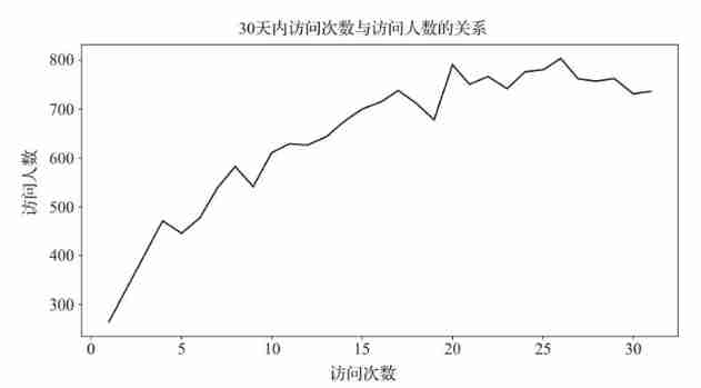
chart 12 30 The relationship between the number of visits in a day and the number of visitors
value_counts(): See how many different values are in a column of the table , And calculate how many duplicate values each different value has in this column .
sort_index(): Sort by the size of a column ,ascending=False It is sorted from large to small .
plt.figure(figsize=(a,b)): Create a palette ,figsize The representative width is a, High for b The graphic , In inches .
plt.ylabel: Set up y Axis ,fontsize Is font size .
plt.xlabel: Set up x Axis .
Pass diagram 12 It can be seen that , The number of users with more visits is higher than that of users with less visits , And in 15 About times is the inflection point , Therefore, the number of visits is defined to be less than or equal to 16 Secondary users are low active users , The number of visits is greater than 16 Secondary users are defined as highly active users , This definition is only from the perspective of users , Work should be defined from a business perspective . The number of visitors with more visits is higher than that with less visits , Contrary to most product access rules , From the side, it reflects the strong user stickiness .
3) Buying activity :
1buy_active_level = labels['counts_30_buy'].value_counts().sort_index(ascending=
 2
 3    False)
 4
 5plt.figure(figsize=(16,9))
 6
 7buy_active_level.plot(title='30 The relationship between the number of purchases in a day and the number of buyers ',fontsize=18)
 8
 9plt.ylabel(' Number of buyers ',fontsize=14)
10
11plt.xlabel(' Number of purchases ',fontsize=14)
12
13labels['buy_active_level'] = ' high '
14
15labels.loc[labels['counts_30_buy']<=14,'buy_active_level'] = ' low '
The result is shown in Fig. 13 Shown .
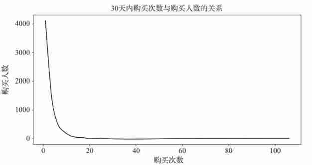
chart 13 30 The relationship between the number of purchases in a day and the number of buyers
From the figure 13 You know ,14 About times is an inflection point , Therefore, it is defined that the number of purchases is less than or equal to 14 Secondary users are low active users , Greater than 14 Secondary users are highly active users .
4) Whether the category purchased is single :
1buy_single=df[df['behavior_type']==4].groupby('user_id').item_category.nunique()
 2
 3.reset_index()
 4
 5buy_single.rename(columns={'item_category':'buy_single'},inplace=True)
 6
 7labels = pd.merge(labels,buy_single,how='left',on='user_id')
 8
 9labels['buy_single'].fillna(-1,inplace=True)
10
11labels['buy_single'] = labels['buy_single'].apply(lambda x: ' yes ' if x>1 else
12
13    ' no ' if x==1 else ' Not purchased ' )
The result is shown in Fig. 14 Shown .
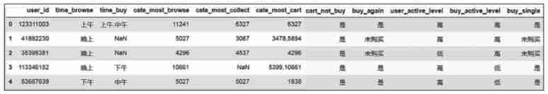
chart 14 Statistics of single purchase category
Understanding the categories that users buy is conducive to building user group behavior , For example, this group accounts for a large proportion of cosmetics consumption , One of the main characteristic labels of this user group is cosmetics .
5) User value grouping (RFM Model ):
1last_buy_days = labels['days_buy'].value_counts().sort_index()
2
3plt.figure(figsize=(16,9))
4
5last_buy_days.plot(title=' The relationship between the number of days since the last purchase and the number of buyers ',fontsize=18)
6
7plt.ylabel(' Number of buyers ',fontsize=14)
8
9plt.xlabel(' Days ago ',fontsize=14)
The result is shown in Fig. 15 Shown .
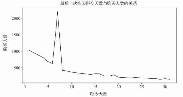
chart 15 The relationship between the number of days before the last purchase and the number of buyers
Use RFM model analysis :
1labels['buy_days_level'] = ' high '
 2
 3labels.loc[labels['days_buy']>8,'buy_days_level'] = ' low '
 4
 5labels['rfm_value'] = labels['buy_active_level'].str.cat(labels['buy_days_level'])
 6
 7def trans_value(x):
 8
 9    if x == ' high ':
10
11        return ' Important value customers '
12
13    elif x == ' Low high ':
14
15        return ' Focus on customers '
16
17    elif x == ' High and low ':
18
19        return ' Important call back customers '
20
21    else:
22
23        return ' About to lose customers '
24
25labels['rfm'] = labels['rfm_value'].apply(trans_value)
26
27#  Here apply() Called a self-defined (def) Function of
28
29labels.drop(['buy_days_level','rfm_value'],axis=1,inplace=True)
30
31labels['rfm'].value_counts()
The result is shown in Fig. 16 Shown .
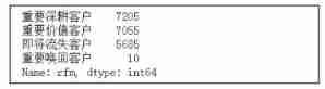
chart 16 RFM Model analysis results
str.cat() It refers to splicing two independent strings , Here will be
'buy_active_level‘ and 'buy_days_level' Splicing . If you want to add a separator between two merged columns , Can be found in cat Add :sep='-', use - Connect and merge content .
take buy_active_level and buy_days_level Combine , formation “ high ” perhaps “ High and low ” etc. . Combine the two important indicators , Every user_id Enter different classification groups .RFM Model is an important tool to measure customer value and customer profitability , among ,R(recently): Last consumption ;F(Frequently): Consumption frequency ;M(Monetary): Consumption amount .
Formulate different marketing strategies for the final output user groups . Pay attention to and maintain important value customers ; For important users , Give corresponding price incentives , Such as discounts and bundling sales, increase the purchase frequency of users , Improve viscosity ; Call back users for important , Stimulate at a specific time point , For example, stimulate the selling points of products 、 Brand instillation, etc , Continue to strengthen their recognition of the brand , Increase loyalty ; For lost customers , In this case , Because its number accounts for about one third , Further analysis is needed to find out the reasons for the loss .
About author : Liu peng , professor , Doctor of Tsinghua University , Cloud computing 、 Well known experts in the field of big data and artificial intelligence , President of Nanjing yunchuang Big Data Technology Co., Ltd 、 Director of AI expert committee of China big data application Alliance . Leader of cloud storage group of cloud computing Expert Committee of China Electronics Society 、 Expert of cloud computing research center of Ministry of industry and information technology .
High school strong , Technical experts in artificial intelligence and big data , Have very deep accumulation , Good at machine learning and natural language processing , Especially deep learning , be familiar with Tensorflow、PyTorch Equal depth learning development framework . Once obtained “2019 National outstanding student in mathematical modeling ”. Participating in the research and development project of New Coronavirus artificial intelligence prediction system guided by academician Zhong Nanshan , Jointly publish academic papers with academician Zhong Nanshan team .
This article is excerpted from 《Python Financial data mining and Analysis Practice 》, Issued under the authority of the publisher .(ISBN:9787111696506)

《Python Financial data mining and Analysis Practice 》
Click on the picture above to learn and buy
Recommended language : Yunchuang big data ( The listed company ) Written by the president , Zero Foundation Institute Financial Data Mining , With case 、 video 、 Code 、 data 、 Exercises and answers .
 present sb. with a book

     Interact with official account in the following ways , You will have the opportunity to receive the above book !
 The way of activity : Reply in the official account background “ Financial data ” Participate in activities , At that time, we will draw... From the participating partners 1 A lucky goose !

     Activity time : By 1 month 24 Japan 20 spot ( Wednesday ) A prize , Be there or be square .
     Get your little partner and get involved ~
Let me know you're watching **
边栏推荐
- 使用 flask_whooshalchemyplus jieba实现flask的全局搜索
- [pointer] the array is stored in reverse order and output
- 指针 --按字符串相反次序输出其中的所有字符
- High concurrency programming series: 6 steps of JVM performance tuning and detailed explanation of key tuning parameters
- My first blog
- 1.支付系统
- 数据库多表链接的查询方式
- 【指针】查找最大的字符串
- STC-B学习板蜂鸣器播放音乐2.0
- What level do 18K test engineers want? Take a look at the interview experience of a 26 year old test engineer
猜你喜欢
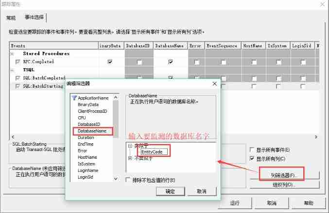
Database monitoring SQL execution
![Transplant hummingbird e203 core to Da Vinci pro35t [Jichuang xinlai risc-v Cup] (I)](/img/85/d6b196f22b60ad5003f73eb8d8a908.png)
Transplant hummingbird e203 core to Da Vinci pro35t [Jichuang xinlai risc-v Cup] (I)
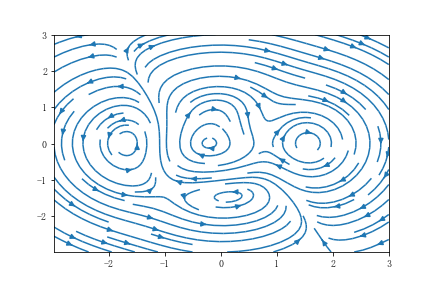
Get started with Matplotlib drawing
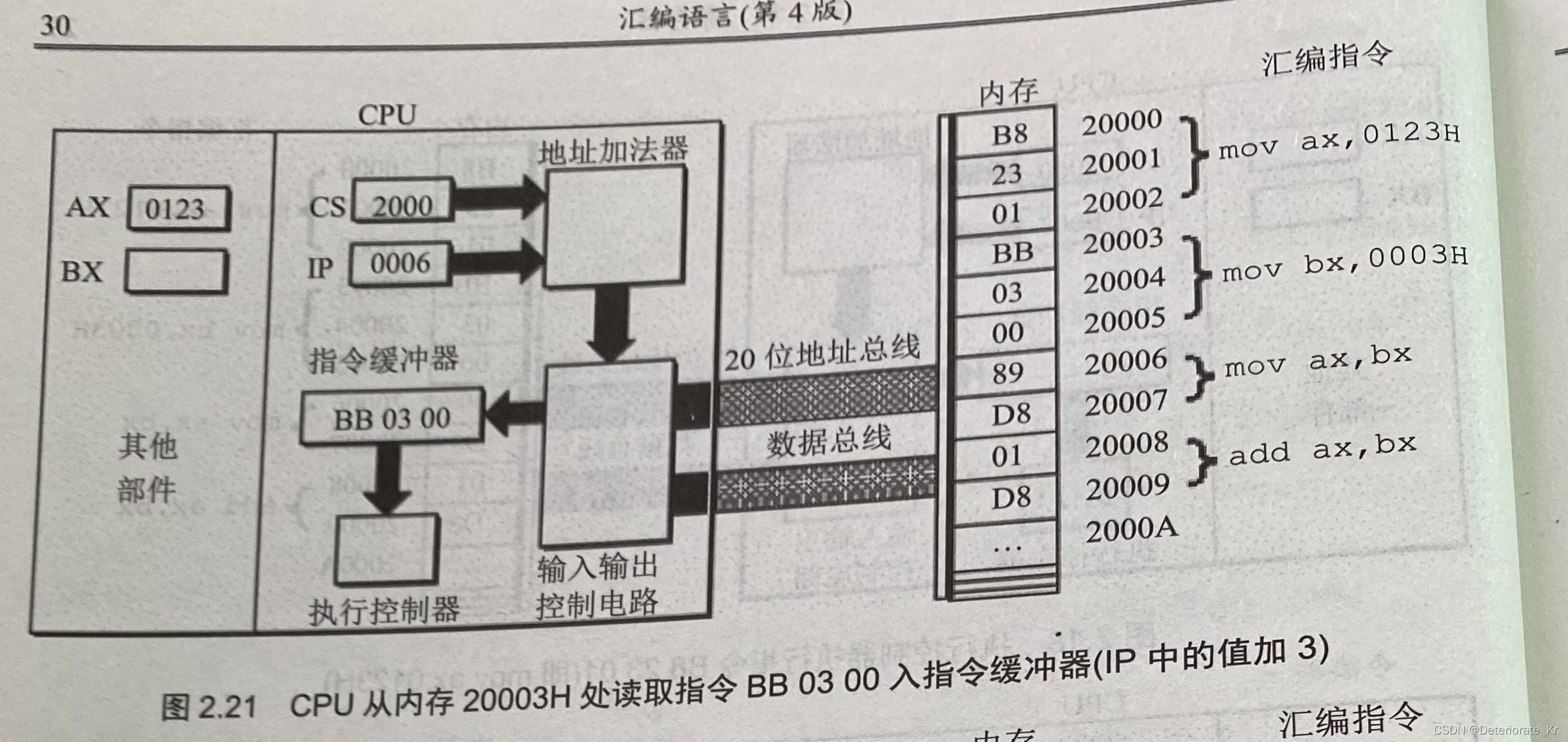
王爽汇编语言详细学习笔记二:寄存器
Login the system in the background, connect the database with JDBC, and do small case exercises

数字电路基础(三)编码器和译码器

四元数---基本概念(转载)

1.支付系统

What is the transaction of MySQL? What is dirty reading and what is unreal reading? Not repeatable?
Wang Shuang's detailed learning notes of assembly language II: registers
随机推荐
Oracle foundation and system table
Zhejiang University Edition "C language programming experiment and exercise guide (3rd Edition)" topic set
Pointer -- eliminate all numbers in the string
Vysor uses WiFi wireless connection for screen projection_ Operate the mobile phone on the computer_ Wireless debugging -- uniapp native development 008
To brush the video, it's better to see if you have mastered these interview questions. Slowly accumulating a monthly income of more than 10000 is not a dream.
Database monitoring SQL execution
[oiclass] maximum formula
{1,2,3,2,5}查重问题
C language do while loop classic Level 2 questions
【指针】查找最大的字符串
Build your own application based on Google's open source tensorflow object detection API video object recognition system (I)
《统计学》第八版贾俊平第四章总结及课后习题答案
Common Oracle commands
《统计学》第八版贾俊平第二章课后习题及答案总结
JDBC 的四种连接方式 直接上代码
Transplant hummingbird e203 core to Da Vinci pro35t [Jichuang xinlai risc-v Cup] (I)
【指针】求解最后留下的人
数字电路基础(一)数制与码制
Soft exam information system project manager_ Project set project portfolio management --- Senior Information System Project Manager of soft exam 025
Build your own application based on Google's open source tensorflow object detection API video object recognition system (II)