当前位置:网站首页>Statistics 8th Edition Jia Junping Chapter XIII Summary of knowledge points of time series analysis and prediction and answers to exercises after class
Statistics 8th Edition Jia Junping Chapter XIII Summary of knowledge points of time series analysis and prediction and answers to exercises after class
2022-07-06 14:31:00 【No two or three things】
Catalog
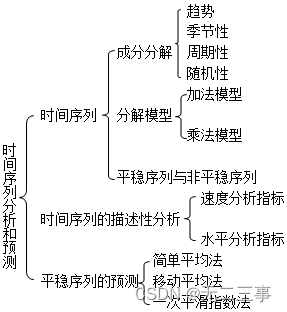
One 、 Knowledge framework
Two 、 Exercises
1 yes 1991~2008 China's fiscal revenue data in . Use exponential curve to predict 2009 Annual revenue , And compare the actual value with the predicted value .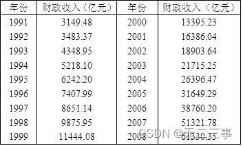
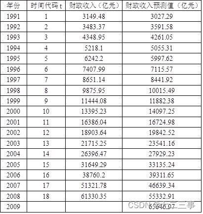
Explain : Let the trend equation of the exponential curve be Yt=b0b1t, Take logarithm at both ends to get ln(Yt)=ln(b0)+tln(b1). According to the principle of least squares , Get ln(b1)=0.1709,ln(b0)=7.8445, The corresponding exponential curve equation is Yt=2551.6615×1.1864t.
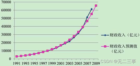
take t=1,2,…,18 Substitute into the trend equation to get the predicted value of each period , take t=19 Substitute into the trend equation to get 2009 The forecast value of annual fiscal revenue . The calculation results are shown in
2 surface 13-6 It's a hotel 18 Monthly turnover data .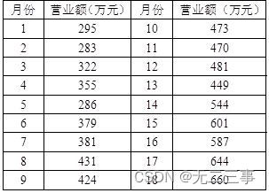
requirement :
(1) use 3 The period moving average method predicts the 19 Monthly turnover .
(2) Use exponential smoothing , Use the smoothing coefficient α=0.3,α=0.4 and α=0.5 Forecast monthly turnover , Analyze the prediction error , Explain which smoothing coefficient is more suitable for prediction .
(3) Establish a trend equation to predict the turnover of each month , Calculate the standard error of estimation .
Explain :(1) The first 19 Months 3 The period moving average forecast value is :
F19=(587+644+660)/3=630.33
(2) from Excel Output exponential smoothing prediction value , As shown in the table .
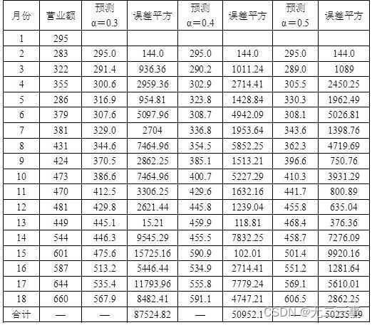
α=0.3 The predicted value is :F19=0.3×660+(1-0.3)×567.9=595.5, Square of error =87524.82
α=0.4 The predicted value is :F19=0.4×660+(1-0.4)×591.1=618.7, Square of error =50952.1
α=0.5 The predicted value is :F19=0.5×660+(1-0.5)×606.5=633.3, Square of error =50235.49 Compare the square of each error ,α=0.5 More appropriate .
(3) According to the least square method , utilize Excel The output regression results are shown in the table .
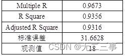
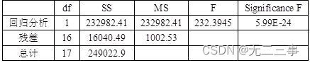
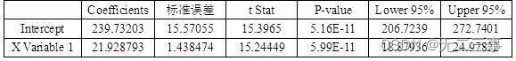
So the linear trend equation is :Yt=239.73+21.9288t; Estimate the standard error SY=31.6628.
3 In our country 1964~1999 Annual yarn production data , As shown in the table 13-11 Shown ( Company : Ten thousand tons of ).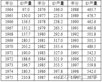
(1) Draw a time series diagram to describe its trend .
(2) Choose a suitable trend line to fit the data , And predict according to the trend line 2000 Annual production .
Explain :(1) Drawing time series , As shown in the figure .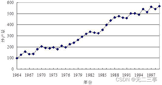
(2) As you can see from the diagram , Yarn output has an obvious linear trend . use Excel The obtained linear trend equation is :Yt=69.5202+13.9495t
therefore 2000 The predicted value is :Y37=69.5202+13.9495×37=585.65( Ten thousand tons of )
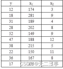
4 Counter table 13-12 The data of are respectively fitted to the linear trend line Yt=b0+b1t、 Second order curve Yt=b0+b1t+b2t2 And third-order curve Yt=b0+b1t+b2t2+b3t3, And compare the results .
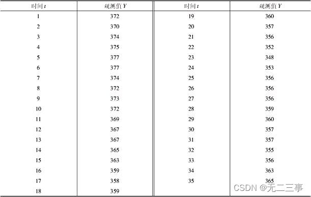 Explain : When finding the second-order curve and the third-order curve , First, linearize it , Then use the least square method to solve according to linear regression . use Excel The obtained trend line 、 Coefficients of second-order curve and third-order curve , As shown in the table .
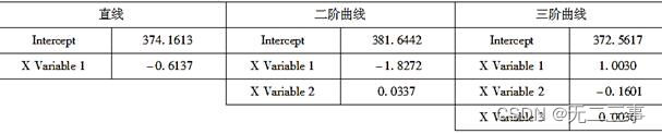
So the trend equations are :
Linear trend :Yt=374.1613-0.6137t
Second order curve :Yt=381.6442-1.8272t+0.0337t2 Third order curve :Yt=372.5617+1.0030t-0.1601t2+0.0036t3
The prediction value and prediction error obtained from the trend equation , As shown in the table .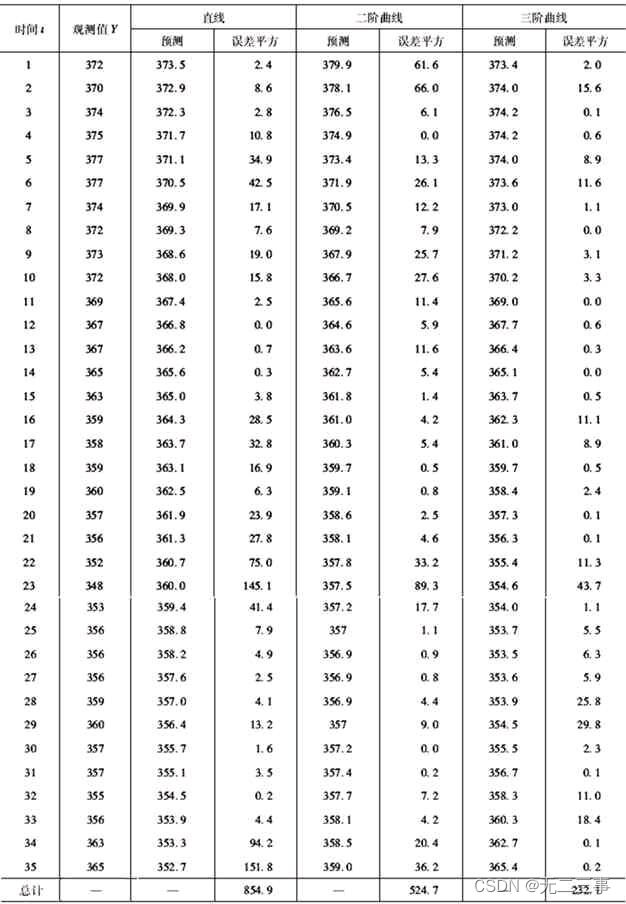
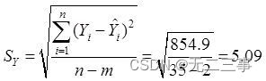
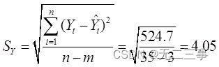
The standard errors of different trend line predictions are :
A straight line :
Second order curve :
Third order curve :
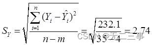
By comparing the prediction errors , The error of the straight line is the largest , The error of the third-order curve is the smallest .
From the prediction diagram of different trend equations ( As shown in the figure ) It can also be seen that , The fitting between the third-order curve and the original sequence is the best .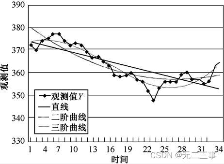
5 A trading company is mainly engaged in the export business of products , In order to reasonably organize the supply , Need to know the changes of export orders . Table is 2011~2015 The amount of export orders in each month of the year ( Company : Ten thousand yuan ).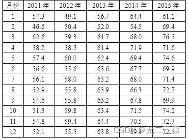
requirement :
(1) Draw a trend chart according to the monthly data of each year , Explain the characteristics of the time series .
(2) Calculate the forecast value of each month , What do you think should be done ?
(3) Choose the appropriate method to predict 2016 year 1 The export order amount of the month .
Explain :(1) Draw a trend chart , As shown in the figure .
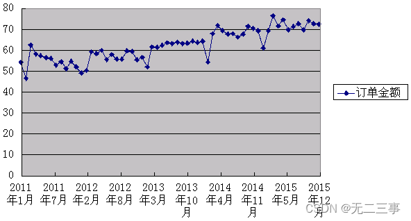
As can be seen from the trend chart , There is no trend in the data of each month of each year , But from 2011~2015 Look at the changes in , There is a certain linear trend in the order amount .
(2) Because it predicts the order amount of each month , Therefore, moving average method or exponential smoothing method is more appropriate .
(3) use Excel use 12 The result predicted by the term moving average method is :F2016/1=71.4( Ten thousand yuan ).
use Excel Use exponential smoothing (α=0.4) The prediction result is :F2016/1=72.5( Ten thousand yuan ).
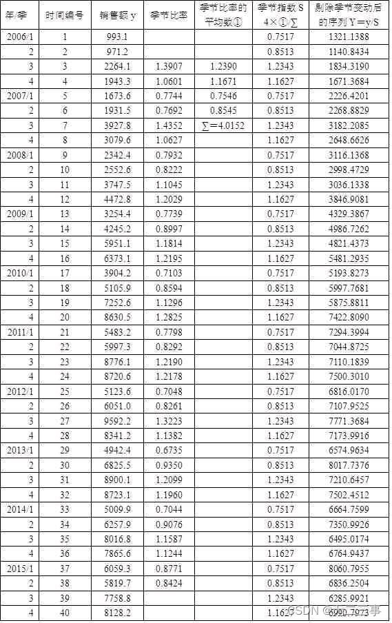
6 surface 13-16 It is the quarterly sales data of a large department store in recent years ( Company : Ten thousand yuan ). Decompose the constituent elements of this time series , Calculate the seasonal index , Excluding seasonal changes , Calculate the trend equation after excluding seasonal changes .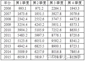
Explain : Calculate the seasonal index by the seasonal average method , Take the moving average number of items equal to the cycle length , namely k=4, Because the number of moving items is even , So we need to do two moving averages .
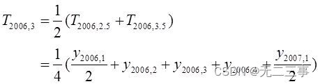
for example :2006 The result of the first moving average in is :
T2006,2.5=(y2006,1+y2006,2+y2006,3+y2006,4)/4
T2006,3.5=(y2006,2+y2006,3+y2006,4+y2006,1)/4
……
Then the result of the second moving average is :
……
namely 2006 In the first 3 The quarterly moving average is :
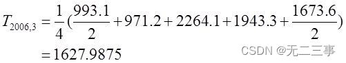
so 2006 In the first 3 The seasonal ratio of the quarter is :
y2006,3/T2006,3=2264.1/1627.9875=1.3907
Empathy 2006 In the first 4 The quarterly moving average is :
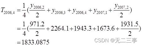
so 2006 In the first 4 The seasonal ratio of the quarter is :
y2006,4/T2006,4=1943.3/1833.0875=1.0601
Similarly, we can get the moving average of other months , Then we can get the corresponding seasonal ratio , Finally, we can get the seasonal index . After calculating the seasonal index , Divide each actual observation by the corresponding seasonal index , So as to eliminate seasonal changes , The formula is :y/S=(T×S×I)/S=T×I. The calculation results are shown in the table .
Draw a seasonal chart , As shown in the figure , It can be seen from the picture that the peak season is 3 quarter , Off season is the first 1 quarter .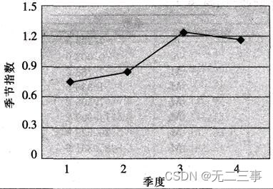
Draw the sales volume and its trend chart after excluding seasonal changes , As shown in the figure .
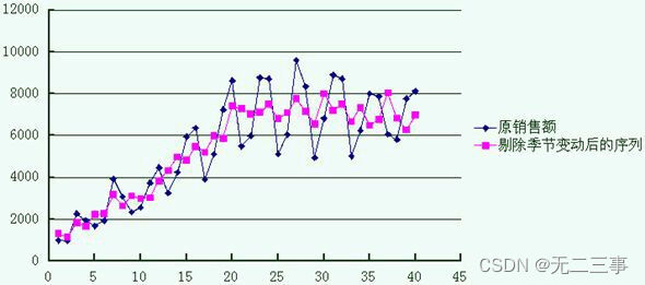
It can be seen from the picture that , One variable linear model can be used to predict the sales of each quarter , Let the trend equation be :Yt=b0+b1t, from Excel Available :b0=2043.92,b1=163.7064. Therefore, the trend equation of sales after excluding seasonal changes is :Yt=2043.92+163.7064t
边栏推荐
- 搭建域环境(win)
- SystemVerilog discusses loop loop structure and built-in loop variable I
- 7-6 local minimum of matrix (PTA program design)
- SQL注入
- Apache APIs IX has the risk of rewriting the x-real-ip header (cve-2022-24112)
- sqqyw(淡然点图标系统)漏洞复现和74cms漏洞复现
- 循环队列(C语言)
- 《英特尔 oneAPI—打开异构新纪元》
- 《统计学》第八版贾俊平第一章课后习题及答案总结
- HackMyvm靶机系列(3)-visions
猜你喜欢
《统计学》第八版贾俊平第九章分类数据分析知识点总结及课后习题答案
关于交换a和b的值的四种方法
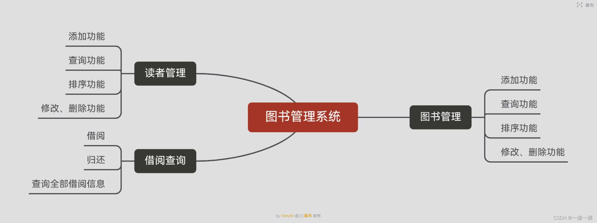
图书管理系统
Statistics 8th Edition Jia Junping Chapter 12 summary of knowledge points of multiple linear regression and answers to exercises after class
关于超星脚本出现乱码问题
记一次edu,SQL注入实战
《统计学》第八版贾俊平第十二章多元线性回归知识点总结及课后习题答案
Intranet information collection of Intranet penetration (4)
搭建域环境(win)
攻防世界MISC练习区(SimpleRAR、base64stego、功夫再高也怕菜刀)
随机推荐
sqqyw(淡然点图标系统)漏洞复现和74cms漏洞复现
2022华中杯数学建模思路
Proceedingjoinpoint API use
中间件漏洞复现—apache
. Net6: develop modern 3D industrial software based on WPF (2)
xray與burp聯動 挖掘
Overview of LNMP architecture and construction of related services
Internet Management (Information Collection)
浙大版《C语言程序设计实验与习题指导(第3版)》题目集
JDBC read this article is enough
servlet中 servlet context与 session与 request三个对象的常用方法和存放数据的作用域。
xray与burp联动 挖掘
Apache APIs IX has the risk of rewriting the x-real-ip header (cve-2022-24112)
Statistics 8th Edition Jia Junping Chapter 3 after class exercises and answer summary
《英特尔 oneAPI—打开异构新纪元》
XSS (cross site scripting attack) for security interview
记一次edu,SQL注入实战
图书管理系统
How to understand the difference between technical thinking and business thinking in Bi?
The difference between layer 3 switch and router