当前位置:网站首页>Numpy Quick Start Guide
Numpy Quick Start Guide
2022-07-06 14:34:00 【ブリンク】
Numpy Quick Start Guide
List of articles
Numpy brief introduction
Numpy yes Python A basic scientific computing library , It provides multidimensional array objects , And various derived objects . Use C Language precompiled code , Vectorized description , bring Numpy It has faster computing speed , Clearer broadcasting (broadcasting) Mechanism makes code simpler , It also means that the probability of making mistakes is lower . In data analysis 、 The field of machine learning ,Numpy Become Python A popular choice .
Through some examples , Let's get started Numpy. Before that , We need to have a certain Python Basics , We will match matplotlib Library for demonstration .
So we need to import before the demo starts
import numpy as np    # Habitually put numpy Shorthand for np
import matplotlib.pyplot as plt
1. Basic attributes
Numpy The core of this is arrays , We first learn how to create an array , Use np.array() Create a one-dimensional array :
>>> a = np.array([1,2,3])
>>> a
array([1,2,3])
We can also create a high-dimensional array :
>>> a = np.array([[1,2,3],[4,5,6],[7,8,9]])
>>> a
array( [[1,2,3],
        [4,5,6],
        [7,8,9]])
We can use Python Of type() Method to directly view the type of the array
>>> type(a)
numpy.ndarray
At this point, we want to know the dimension of the created array , Then you can check ndarray Class ndim attribute
>>> a.ndim
2
Returns the dimension of the array , It can be understood as [] The number of
At this point, we want to know what shape the created array is , Even with this simple array, we can count it as 3*3 Of , You can see ndarray Medium shape attribute
>>> a.shape
(3,3)
At this point, we want to know how many elements are in this array , You can see ndarray Properties of size
>>> a.size
9
In fact, it is equal to shape Product of attributes
At this point, we want to know what type of elements are stored in the array , You can see ndarray Of dtype attribute
>>> a.dtype
dtype('int32')
numpy.int32, numpy.int16 as well as numpy.float64 Is such as Numpy Some additional types provided , Of course, when creating arrays , You can also use Python The type of data that comes with it .
At this point, we want to know how many bytes each element in the array element occupies , You can see ndarray Of itemsize attribute
>>> a.itemsize
4
actually int32 The byte occupation of type is 32/8=4, And if it is float64 Type elements , Then for 64/8=8 byte
2. How arrays are created
There are many ways to create arrays , The above is given by Python The way of creating arrays by lists and tuples should be noted , The data we give must be included in [] in , Not a column of numbers
>>> a = np.array(1,2,3) #  This is wrong
>>> a = np.array([1,2,3]) #  That's right
When we create an array , You can specify the type of data , Directly in array() Set the dtype The parameter is the desired type
>>> a = np.array([1,2,3,4], dtype = np.complex)
>>> a
array([1.+0.j, 2.+0.j, 3.+0.j, 4.+0.j])
>>> a.dtype
dtype('complex128')
Usually , We don't know what the data in the array is , But I know its size (size), We can initialize these arrays in advance with a fixed size :
zeros() You can create an array of a specified size , All the elements in the array are 0
>>> a = np.zeros((2,3))
>>> a
array([[0., 0., 0.],
       [0., 0., 0.]])
ones() You can create an array of a specified size , All the elements in the array are 1, Of course, when they are created , You can also specify the data type of the element
>>> a = np.ones((3,2), dtype = np.int32)
>>> a
array([[1, 1],
       [1, 1],
       [1, 1]])
We can also use empty() To create an empty array of a specified size , The data inside is randomly generated , This is related to the state of memory
>>> np.empty((2,2,2))
array([[[4.94065646e-324, 2.12199579e-314],
        [4.24399158e-314, 2.12199579e-314]],

       [[6.36598737e-314, 4.24399158e-314],
        [2.12199579e-314, 4.94065646e-324]]])
We can create arrays with certain regularity , Use arange(), It is associated with Python Of range() It's very similar
>>> np.arange(0, 10, 2)
array([0, 2, 4, 6, 8])
>>> np.arange(1,2,0.2)
array([1. , 1.2, 1.4, 1.6, 1.8])
Use arange() One drawback is , We don't know how many elements are stored in the array , Use linspace Can solve this problem , It can directly generate the number of elements you specify .
>>> np.linspace(0,3,6) #  Generate 0-3 Evenly distributed in the middle 6 Number
array([0. , 0.6, 1.2, 1.8, 2.4, 3. ])
3. Insert 、 Sort and remove array elements
You can continue to insert data into the established array , Use insert() Method , The first parameter indicates in which array to insert , The second parameter represents the index , The third parameter represents the inserted value ( It can also be an array ),axis You can specify which direction it is :
>>>a = np.array([[1,2,3,4], [5,6,7,8], [9,10,11,12]])
>>> np.insert(a,1,999,axis=1) #  stay a Array index 1 Insert 999
array([[  1, 999,   2,   3,   4],
       [  5, 999,   6,   7,   8],
       [  9, 999,  10,  11,  12]])
Numpy Medium sort() Method can directly sort elements
>>> a = np.array([5,4,1,2,7,9,3,6,0])
>>> a
array([5, 4, 1, 2, 7, 9, 3, 6, 0])
>>> np.sort(a)
array([0, 1, 2, 3, 4, 5, 6, 7, 9])
Use argsort Method can output the sorted index as an array :
>>> np.argsort(a)
array([8, 2, 3, 6, 1, 0, 7, 4, 5], dtype=int64)
Use delete() Method can delete the elements in the array , How to use it and insert() The method is similar , Just don't enter the third parameter —— value (value)
>>>np.delete(a,[1],axis=0) #  Delete a The second line of the array
array([[ 1,  2,  3,  4],
       [ 9, 10, 11, 12]])
4. Changing the shape of an array
We can go through ndarray Of reshape() Method to change the shape of the array
>>> a = np.arange(12)
>>> a
array([ 0,  1,  2,  3,  4,  5,  6,  7,  8,  9, 10, 11])
>>> a.reshape(4,3) #  Change the array to 4*3
array([[ 0,  1,  2],
       [ 3,  4,  5],
       [ 6,  7,  8],
       [ 9, 10, 11]])
It can be changed to a higher dimension
>>> a.reshape(2,2,3)
array([[[ 0,  1,  2],
        [ 3,  4,  5]],

       [[ 6,  7,  8],
        [ 9, 10, 11]]])
5. Basic operation
We can perform a series of mathematical operations on arrays , Including addition, subtraction, multiplication, division and power operation
>>> a = np.array([1,2,3,4])
>>> b = np.array([8,7,6,5])
>>> b-a
array([7, 5, 3, 1])
>>> a+b
array([9, 9, 9, 9])
>>> a*b
array([ 8, 14, 18, 20])
>>> a/b
array([0.125     , 0.28571429, 0.5       , 0.8       ])
>>> a**2
array([ 1,  4,  9, 16], dtype=int32)
You can see , When doing these operations , It will operate on each corresponding element of the array .Numpy have access to @ @ @ perhaps d o t dot dot Multiply two matrices , The result obtained is the result of matrix multiplication .
>>> a = np.array([[1,2],[3,4]])
>>> b = np.array([[3,2],[1,2]])
>>> [email protected] #  Matrix multiplication
array([[ 5,  6],
       [13, 14]])
>>> a.dot(b)
array([[ 5,  6],
       [13, 14]])
It is worth noting that , When we operate on two different types of arrays , The resulting array will be projected upwards (upcasting), in other words , It will convert data types with low accuracy into types with high accuracy . Here's an example :
>>> a = np.array([[1,2],[3,4]],dtype=np.int32)
>>> b = np.array([[3,2],[1,2]],dtype=np.float64)
>>> c = a + b
>>> c.dtype
dtype('float64')
We can use min() Find the smallest number in the array , Use max() Find the largest number in the array , Use sum() Sum all the elements in the array , Use mean() Average the elements in the array .
>>> a = np.random.random((2,3)) #  produce 2*3 The random number
>>> a
array([[0.09291709, 0.36686894, 0.88096043],
       [0.20985186, 0.1433596 , 0.67468045]])
>>> a.min()
0.09291709064299836
>>> a.max()
0.8809604347992017
>>> a.sum()
2.3686383681150147
>>> a.mean()
0.39477306135250245
Sometimes we want to know some numerical characteristics of a specific row or column , We need to add parameters to these methods axis, When axis=0 When, it means that the columns of the array will be operated on ; And when axis=1 when , The rows of the array will be manipulated , Here's an example :
>>> a = np.arange(12).reshape((3,4))
>>> a
array([[ 0,  1,  2,  3],
       [ 4,  5,  6,  7],
       [ 8,  9, 10, 11]])
>>> a.sum(axis = 0) #  Operate on Columns
array([12, 15, 18, 21])
>>> a.max(axis = 1)
array([ 3,  7, 11]) #  Operate on the line
There is also a special operation : Add up . It is to output the result after adding each element from the first element , It can also be used axis Control row operation or column operation
>>> a = np.arange(12).reshape((3,4))
>>> a
array([[ 0,  1,  2,  3],
       [ 4,  5,  6,  7],
       [ 8,  9, 10, 11]])
>>> a.cumsum()
array([ 0,  1,  3,  6, 10, 15, 21, 28, 36, 45, 55, 66], dtype=int32)
6. Common formula
In mathematics , We often calculate some, such as c o s cos cos, s i n sin sin, t a n tan tan, e n e^n en, x \sqrt{x} x Such operations ,Numpy It can also realize the calculation of these mathematical functions
>>> a = np.arange(4)
>>> a
array([0, 1, 2, 3])
>>> np.sin(a)
array([0.   , 0.84147098, 0.90929743, 0.14112001]) #  Sine function
>> np.exp(a)
array([ 1.   ,  2.71828183,  7.3890561 , 20.08553692]) # e Exponential function
>> np.sqrt(a)
array([0.   , 1.   , 1.41421356, 1.73205081]) #  Root operation
>> np.add(a,a)
array([0, 2, 4, 6]) #  Add operation
There are other formulas that are not used so much , If you will use , You can refer to the relevant information .
7. Indexes 、 Slicing and iteration
The slicing method of one-dimensional array and Python The list is basically similar .
We can go directly through :
Count Group name [ Cable lead Number ] Array name [ Reference no. ] Count Group name [ Cable lead Number ] Index in a way
Count Group name [ rise beginning Cable lead : junction beam Cable lead : Cable lead between Partition ] Array name [ Starting index : End index : Index interval ] Count Group name [ rise beginning Cable lead : junction beam Cable lead : Cable lead between Partition ] Slice in the way of , If you do not fill in the start index and end index , It is considered to be the beginning and the end ; If you do not fill in the index interval , The default is 1
have access to f o r for for Loop through iterations
>>> a = np.arange(10)
>>> a
array([0, 1, 2, 3, 4, 5, 6, 7, 8, 9])
>>> a[3] #  Index to 3 The elements of
3
>>> a[2:8] #  Index to 2-8 The elements of , barring 8
array([2, 3, 4, 5, 6, 7])
>>> a[::3] #  Every time 3 Index is retrieved once
array([0, 3, 6, 9])
>>> for i in a:
...     print(i,end=" ")
0 1 2 3 4 5 6 7 8 9
Certain conditions can also be used for indexing
>>> a[a>5]
array([6, 7, 8, 9])
Each dimension of a multidimensional array has an index , They can be represented by tuples
have access to
Count Group name [ One dimension Cable lead ] [ Two dimension Cable lead ] . . . [ n dimension Cable lead ] Array name [ One dimensional index ][ Two dimensional index ]...[n Vesuoyi ] Count Group name [ One dimension Cable lead ][ Two dimension Cable lead ]...[n dimension Cable lead ] Index in a way
When slicing , Each dimension can be indexed like a one-dimensional array
Count Group name [ ( One dimension ) rise beginning Cable lead : junction beam Cable lead : Cable lead between Partition , ( Two dimension ) rise beginning Cable lead : junction beam Cable lead : Cable lead between Partition , . . . , ( n dimension ) rise beginning Cable lead : junction beam Cable lead : Cable lead between Partition ] Array name [( A one-dimensional ) Starting index : End index : Index interval ,( A two-dimensional ) Starting index : End index : Index interval ,...,(n dimension ) Starting index : End index : Index interval ] Count Group name [( One dimension ) rise beginning Cable lead : junction beam Cable lead : Cable lead between Partition ,( Two dimension ) rise beginning Cable lead : junction beam Cable lead : Cable lead between Partition ,...,(n dimension ) rise beginning Cable lead : junction beam Cable lead : Cable lead between Partition ]
Look directly at the following example :
>>> def f(x, y):
...     return 5*x+y
>>> a = np.fromfunction(f,(4,4),dtype = np.int64
>>> #  Create an array from a function ,x and y Are the values of the index
array([[ 0,  1,  2,  3],
       [ 5,  6,  7,  8],
       [10, 11, 12, 13],
       [15, 16, 17, 18]], dtype=int64)
>>> a[3,2]
17
>>> a[:,1:3]
array([[ 1,  2],
       [ 6,  7],
       [11, 12],
       [16, 17]], dtype=int64)
It should be noted that if you pass -1, The last element or column will be displayed / That's ok
>>> a[1][-1]
8
At iteration time , The multidimensional array iterates over the first dimension , If we want to iterate over elements , You can use f l a t flat flat To flatten
>>> for row in a:
...        print(row)
[0 1 2 3]
[5 6 7 8]
[10 11 12 13]
[15 16 17 18]
>>> for elm in a.flat:
...    print(elm,end=" ")
0 1 2 3 5 6 7 8 10 11 12 13 15 16 17 18
8. Inversion of array
Arrays can perform some special changes , Let's demonstrate directly
>>> a = np.random.randint(8,size=(2,4))
>>> a
array([[3, 7, 7, 5],
       [6, 6, 1, 7]])
>>> a.shape
(2, 4)
>>> a.ravel() #  Flattening   You can also use flatten()
array([3, 7, 7, 5, 6, 6, 1, 7])
>>> a.flatten()
array([3, 7, 7, 5, 6, 6, 1, 7])
>>> a.T #  Transpose the array
array([[3, 6],
       [7, 6],
       [7, 1],
       [5, 7]])
''' reshape and resize The difference is that  resize Will change the shape of the current variable   and reshape Will not be  '''
>>> a.resize((2,4))
>>> a
array([[3, 7, 7, 5],
       [6, 6, 1, 7]])
>>> a.reshape(1,8)
array([[3, 7, 7, 5, 6, 6, 1, 7]])
>>> a
array([[3, 7, 7, 5],
       [6, 6, 1, 7]])
If one of the parameters of the shape has been determined , Then another parameter can be set to -1, It will automatically calculate the value
>>> a = np.randint(1000,size = (10*100))
>>> b = a.reshape(25,-1)
>>> b.shape
(25, 40)
8. Stack of arrays
Numpy You can stack some arrays from different directions
>>> a = np.zeros((2,2))
>>> b = np.ones((2,2))
>>> np.vstack((a,b)) #  The stack of columns
array([[0., 0.],
       [0., 0.],
       [1., 1.],
       [1., 1.]])
>>> np.hstack((a,b)) #  Line stacking
array([[0., 0., 1., 1.],
       [0., 0., 1., 1.]])
9. Segmentation of arrays
By using hsplit, You can slice a larger array horizontally into smaller arrays , And put back the array of the specified size
>>> a = np.random.randint(20,size=(2,10))
>>> a
array([[17,  0,  4, 16,  0, 11,  1,  0,  7,  7],
       [ 8,  9,  4,  0, 15,  5, 16,  3,  1, 16]])
>>> np.hsplit(a,2) #  take a The array is divided into two arrays
[array([[17,  0,  4, 16,  0],
        [ 8,  9,  4,  0, 15]]),
 array([[11,  1,  0,  7,  7],
        [ 5, 16,  3,  1, 16]])]
>>> np.hsplit(a,(2,5)) #  from 2 and 5 Division a Array
[array([[17,  0],
        [ 8,  9]]),
 array([[ 4, 16,  0],
        [ 4,  0, 15]]),
 array([[11,  1,  0,  7,  7],
        [ 5, 16,  3,  1, 16]])]
Similar to this ,vsplit() and hsplit() In the same way , Just split along the vertical axis . and array_split() You need to specify which axis to split along .
>>> a = np.random.randint(48,size=(6,8))
>>> a
array([[29, 14, 16, 44, 35,  4, 13, 18],
       [12, 31, 15,  6, 12, 45,  3, 41],
       [28, 11, 29,  3, 31, 20, 29, 41],
       [30,  1, 21, 21, 13,  2, 45,  6],
       [43, 47,  0, 41, 41, 23, 38, 38],
       [16,  3, 18, 28, 43, 45, 38,  1]])
>>> np.vsplit(a,2)
[array([[29, 14, 16, 44, 35,  4, 13, 18],
        [12, 31, 15,  6, 12, 45,  3, 41],
        [28, 11, 29,  3, 31, 20, 29, 41]]),
 array([[30,  1, 21, 21, 13,  2, 45,  6],
        [43, 47,  0, 41, 41, 23, 38, 38],
        [16,  3, 18, 28, 43, 45, 38,  1]])]
>>> np.array_split(a,(2,5),axis=0)
[array([[29, 14, 16, 44, 35,  4, 13, 18],
        [12, 31, 15,  6, 12, 45,  3, 41]]),
 array([[28, 11, 29,  3, 31, 20, 29, 41],
        [30,  1, 21, 21, 13,  2, 45,  6],
        [43, 47,  0, 41, 41, 23, 38, 38]]),
 array([[16,  3, 18, 28, 43, 45, 38,  1]])]
10. Copy of array
There are three cases of replication : No duplication , Light copy and deep copy
(1) No duplication
>>> a = np.array([[1,2],[3,4]])
>>> b = a #  No new objects are created
>>> b is a # a and b Just the name of an array class
True
(2) A shallow copy
Different array objects can share the same data ,view() Method provides a possibility to create such an array
>>> c = a.view()
>>> c
array([[1, 2],
       [3, 4]])
>>> c is a
False
>>> c.base is a
True
>>> c = c.reshape((1, 4))
>>> c.shape
(1, 4)
>>> a.shape # a The shape of has not changed
(2, 2)
>>> c[0,0]=666
>>> a # a That's changed
array([[666,   2],
       [  3,   4]])
(3) Deep copy
Numpy Provided copy() Method can make a complete copy .
Let's look at an example
>>> d = a.copy()
>>> d is a # d and a Two objects
False
>>> d.base is a # d and a Don't share any data
False
>>> d[0][0] = 999
>>> a # a The value in does not change
array([[666,   2],
       [  3,   4]])
Sometimes , When we copied a sliced array , The original array has no value , So you can delete it directly
>>> e = a[:,1].copy()
>>> del a
11. radio broadcast (Broadcasting)
The broadcast mechanism can make some arrays with different input shapes meaningful in the above operations . The broadcasting mechanism has the following rules :
a. Let all the input arrays look to the array with the longest shape , The insufficient parts in the shape are all preceded by 1 A filling .
b. The shape of the output array is the maximum value on each dimension of the shape of the input array .
c. If a dimension of the input array has the same length as the corresponding dimension of the output array, or its length is 1 when , This array can be used to calculate , Otherwise mistakes .
d. When the length of a dimension of the input array is 1 when , The first set of values on this dimension is used when calculating along this dimension .
In short , The broadcast will expand the array that cannot be calculated into the array that can be calculated
>>> a = np.array([[ 0, 0, 0],[10,10,10]])
>>> b = np.array([1,2,3])
>>> a + b
array([[ 1,  2,  3],
       [11, 12, 13]])
*12. Advanced indexing and indexing techniques
(1) Array to index the array
An array can be used as an index of an array , Look directly at the example
>>> a = np.arange(10)**2 #  An array of the first ten squares
>>> a
array([ 0,  1,  4,  9, 16, 25, 36, 49, 64, 81], dtype=int32)
>>> index = np.array([1,3,4,6]) #  Define an index array
>>> a[index]
array([ 1,  9, 16, 36], dtype=int32)
>>> j = np.array([[3, 4], [9, 7]]) #  Define a two-dimensional index array
>>> a[j] #  The result is the sum of j The shape of the array is consistent
array([[ 9, 16],
       [81, 49]], dtype=int32)
(2) An array of Boolean element types
An array of boolean type can be used as the index of another array of the same shape , If the index is True, The output , If the index is False, No output .
>>> a = np.arange(12).reshape(3,4)
>>> b = a > 6
>>> b
array([[False, False, False, False],
       [False, False, False,  True],
       [ True,  True,  True,  True]])
>>> a[b]
array([ 7,  8,  9, 10, 11])
边栏推荐
- 《统计学》第八版贾俊平第四章总结及课后习题答案
- The most popular colloquial system explains the base of numbers
- [issue 18] share a Netease go experience
- 1.支付系统
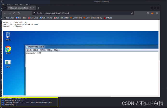
- MSF generate payload Encyclopedia
- On the idea of vulnerability discovery
- Interview Essentials: what is the mysterious framework asking?
- 《统计学》第八版贾俊平第十章方差分析知识点总结及课后习题答案
- 《统计学》第八版贾俊平第十一章一元线性回归知识点总结及课后习题答案
- 指针 --按字符串相反次序输出其中的所有字符
猜你喜欢
Statistics 8th Edition Jia Junping Chapter 14 summary of index knowledge points and answers to exercises after class
Résumé des points de connaissance et des réponses aux exercices après la classe du chapitre 7 de Jia junping dans la huitième édition des statistiques
Intranet information collection of Intranet penetration (4)
《统计学》第八版贾俊平第六章统计量及抽样分布知识点总结及课后习题答案
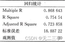
Statistics, 8th Edition, Jia Junping, Chapter 11 summary of knowledge points of univariate linear regression and answers to exercises after class

Low income from doing we media? 90% of people make mistakes in these three points
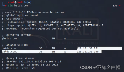
外网打点(信息收集)
内网渗透之内网信息收集(二)
Internet Management (Information Collection)
![New version of postman flows [introductory teaching chapter 01 send request]](/img/0f/a41a39093a1170cc3f62075fd76182.jpg)
New version of postman flows [introductory teaching chapter 01 send request]
随机推荐
Sword finger offer 23 - print binary tree from top to bottom
Statistics 8th Edition Jia Junping Chapter 7 Summary of knowledge points and answers to exercises after class
Markdown font color editing teaching
2022华中杯数学建模思路
Résumé des points de connaissance et des réponses aux exercices après la classe du chapitre 7 de Jia junping dans la huitième édition des statistiques
Mysql的事务是什么?什么是脏读,什么是幻读?不可重复读?
Wu Enda's latest interview! Data centric reasons
记一次api接口SQL注入实战
captcha-killer验证码识别插件
浅谈漏洞发现思路
XSS (cross site scripting attack) for security interview
Windows platform mongodb database installation
线程的实现方式总结
Overview of LNMP architecture and construction of related services
How to understand the difference between technical thinking and business thinking in Bi?
【指针】求字符串的长度
“人生若只如初见”——RISC-V
Intranet information collection of Intranet penetration (I)
What language should I learn from zero foundation. Suggestions
Intranet information collection of Intranet penetration (4)