当前位置:网站首页>Chapter 16 intensive learning
Chapter 16 intensive learning
2022-07-08 01:07:00 【Intelligent control and optimization decision Laboratory of Cen】
1. Analyze the connection and difference between reinforcement learning and supervised learning .
What a machine has to do is to learn one by constantly trying in the environment " Strategy " (policy) π \pi π, According to this strategy , In state x x x Next, you can know what action to perform α = π ( x ) \alpha=\pi(x) α=π(x), For example, when you see that the melon seedling state is lack of water , Can return to action " watering ". There are two ways to represent a strategy : One is to represent the strategy as a function π : X ↦ A \pi:X \mapsto A π:X↦A, Deterministic strategies are often expressed in this way ; The other is probability representation π : X × A ↦ R \pi:X\times A\mapsto\mathbb{R} π:X×A↦R
Randomness strategy is often expressed in this way , π ( x , a ) \pi(x ,a) π(x,a) For state x x x Choose action a a a Probability , It has to be here ∑ a π ( x , a ) = 1 \sum_{a}^{}\pi(x,a)=1 ∑aπ(x,a)=1.
If the " state " It corresponds to " Example "、“ action " Corresponding to " Mark " You can see , Strengthen learning " Strategy " In fact, it is equivalent to supervising learning " classifier ” ( When the action is discrete ) or " Regressor " ( When the action is continuous , There is no difference in the form of the model . But the difference is , In reinforcement learning, there is no labeled sample in supervised learning ( namely " Example - Mark " Yes ) , In other words , No one directly tells the machine what action it should do under what state , Only when the final result is announced , Can pass " reflection " Whether the previous action is correct to learn . therefore , Reinforcement learning can be regarded as having " Delay flag information " The problem of supervised learning .
2. ϵ \epsilon ϵ- How can the greedy method achieve the balance between exploration and utilization .
ϵ \epsilon ϵ- The greedy method is based on a probability to make a compromise between exploration and utilization : Every time you try , With ϵ \epsilon ϵ To explore the probability of , In other words, a rocker arm is randomly selected with uniform probability ; With 1 − ϵ 1-\epsilon 1−ϵ The use of probability , That is to choose the one with the highest average reward at present .
If the uncertainty of rocker arm reward is large , For example, when the probability distribution is wide , More exploration is needed , At this time, a larger ϵ \epsilon ϵ value ; If the uncertainty of the rocker arm is small , For example, when the probability distribution is relatively concentrated , Then a few attempts can well approximate the real reward , What is needed at this time ϵ \epsilon ϵ smaller . Usually make ϵ \epsilon ϵ Take a smaller constant , Such as 0.1 or 0.01. However , If the number of attempts is very large , So after a period of time , The rewards of the rocker arm can be well approximated , No need to explore , In this case ϵ \epsilon ϵ As the number of attempts increases, it gradually decreases , For example, Ling ϵ = 1 / t \epsilon=1/ \sqrt{t} ϵ=1/t.
3. How to use gambling machine algorithm to realize reinforcement learning task .
Different from general supervised learning , The final reward of reinforcement learning task can only be observed after multi-step action . Reinforcement learning is significantly different from supervised learning , Because the machine tries to find the results of each action , There is no training data to tell the machine which action to do .
Consider simpler situations : Maximize one-step rewards , That is, consider one-step operation . actually , One step reinforcement learning task corresponds to a theoretical model , namely “K- Swing arm gambling machine ”. As shown in the figure below ,K- There are K A rocker arm , After putting in a coin, the gambler can choose to press one of the rocker arms , Each rocker gives out a coin with a certain probability , But this probability gambler doesn't know . The goal of gamblers is to maximize their rewards through certain strategies , That is to get the most coins .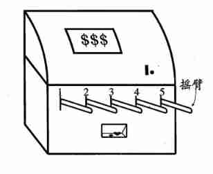
If only to know the expected reward of each rocker arm , You can use “ Just explore ” Law : Distribute all the trial opportunities equally to each rocker arm , Finally, the average payout probability of each rocker arm is taken as the approximate estimation of its reward expectation . If only to perform the action with the greatest reward , You can use “ Use only ” Law : Press the best rocker arm at present , If there are more than one rocker arm, it is optimal , Then randomly choose one of them . obviously ,“ Just explore ” The method can estimate the reward of each rocker arm very well , But you will lose a lot of opportunities to choose the best rocker arm ;“ Use only ” The law is the opposite , It doesn't expect rewards well , It is likely that the optimal rocker arm is often not achieved . therefore , Neither of these methods can maximize the final cumulative reward . obviously , If you want to accumulate the most rewards , We must reach a good compromise between exploration and utilization .
4. Trial derivation The full probability expansion of discount cumulative reward (16.8).
When the model is known , For any strategy π \pi π Can estimate the expected cumulative rewards brought by this strategy . Let function V π ( x ) V^{\pi}(x) Vπ(x) Represents slave state x x x set out , Executive action a a a Then use the strategy π \pi π Cumulative rewards ; function Q π ( x , a ) Q^{\pi}(x,a) Qπ(x,a) Represents slave state x x x set out , Executive action a a a Then use the strategy π \pi π Cumulative rewards . there V ( ⋅ ) V(\cdot) V(⋅) be called “ State value function ”, Q ( ⋅ ) Q(\cdot) Q(⋅) be called “ state - Action value function ”, Respectively means to specify “ state ” And specify “ state - action ” Cumulative rewards on .
By the definition of cumulative rewards , Stateful valued function 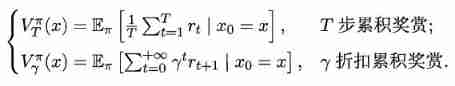
Make x 0 x_{0} x0 Indicates the starting state , a 0 a_{0} a0 Indicates the first action taken in the initial state ; about T T T Step to accumulate rewards , Use subscript t t t Indicates the number of subsequent steps . We are in a state - Action value function 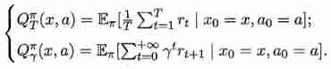
because MDP It has Markov property , That is, the state of the system at the next time is only determined by the state at the current time , Not dependent on any previous state , So the value function has a very simple recursive form . about T T T Step cumulative rewards are 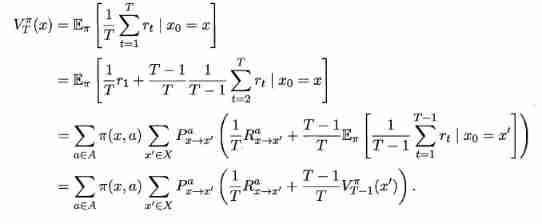
Allied , about γ \gamma γ The cumulative rewards of discounts are 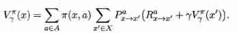
Here's the thing , Formally due to P P P and R R R It is known that , Then the full probability expansion can be carried out .
5. What is the optimality principle in dynamic programming , What does it have to do with strategy updating in reinforcement learning
The key of the dynamic method is to correctly summarize the basic recurrence relations and appropriate boundary conditions . Do that , The problem process must first be divided into several interrelated stages , Properly select state variables and decision variables and define the optimal value function , Thus, a big problem can be transformed into a group of sub problems of the same type , Then solve them one by one . That is, starting from the boundary conditions , Step by step recursive optimization , In the solution of each subproblem , Both use the optimization results of its front subproblem , In turn , The optimal solution of the last subproblem , Is the optimal solution of the whole problem .
Reinforcement learning can refer to the idea of dynamic programming , Just maximize the reward for each step , Can achieve the goal of maximizing cumulative rewards .
6. Complete timing difference learning Chinese (16.31) The derivation of .
The essence of Monte Carlo reinforcement learning , It is an approximation of the expected cumulative reward by averaging after many attempts , But when it is averaged, it is “ Batch processing ” On going , That is, after a complete sampling track is completed, all States - Action update . In fact, this update process can be carried out incrementally . For the State - The action is right ( x , a ) (x,a) (x,a), It may be assumed that based on t t t Samples have estimated the value function Q t π ( x , a ) = 1 t ∑ i = 1 t r i Q_{t}^{\pi}(x,a)=\frac{1}{t}\sum_{i=1}^{t}r_i Qtπ(x,a)=t1∑i=1tri, Then get the t + 1 t+1 t+1 Individual sampling r t + 1 r_{t+1} rt+1 when , Yes :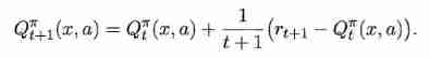
obviously , Just give Q t π ( x , a ) Q_{t}^{\pi}(x,a) Qtπ(x,a) Plus the increment 1 t + 1 ( r ( t + 1 ) − Q t π ( x , a ) ) \frac{1}{t+1}(r_(t+1)-Q_{t}^{\pi}(x,a)) t+11(r(t+1)−Qtπ(x,a)).
A more general , take 1 t + 1 \frac{1}{t+1} t+11 Replace with a coefficient α t + 1 {\alpha}_{t+1} αt+1, The incremental item can be written α ( r t + 1 − Q t π ( x , a ) ) \alpha(r_{t+1}-Q_{t}^{\pi}(x,a)) α(rt+1−Qtπ(x,a)).
With γ \gamma γ Take discount cumulative rewards as an example , Use the dynamic programming method and consider the use of state when the model is unknown - Action value function is more convenient , Available :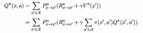
By incremental summation :
among x ′ x^{'} x′ It was the last time in the state x x x Executive action a a a After the transition to the state of , a ′ a^{'} a′ It's a strategy π \pi π stay x ′ x^{'} x′ Action selected on .
7. For goal driven reinforcement learning tasks , The goal is to reach a certain state , For example, the robot walks to the predetermined position , Suppose the robot can only move in one-dimensional space , That is, it can only move left or right , The starting position of the robot is on the far left , The predetermined position is on the far right , Try to set reward rules for such tasks , And programming .
( Procedure reference :https://github.com/MorvanZhou/Reinforcement-learning-with-tensorflow/blob/master/contents/1_command_line_reinforcement_learning/treasure_on_right.py)
边栏推荐
- Vs code configuration latex environment nanny level configuration tutorial (dual system)
- 5. Over fitting, dropout, regularization
- Su embedded training - Day7
- Saving and reading of network model
- [deep learning] AI one click to change the sky
- German prime minister says Ukraine will not receive "NATO style" security guarantee
- Su embedded training - Day6
- Where is the big data open source project, one-stop fully automated full life cycle operation and maintenance steward Chengying (background)?
- v-for遍历元素样式失效
- C# ?,?.,?? .....
猜你喜欢
12. RNN is applied to handwritten digit recognition
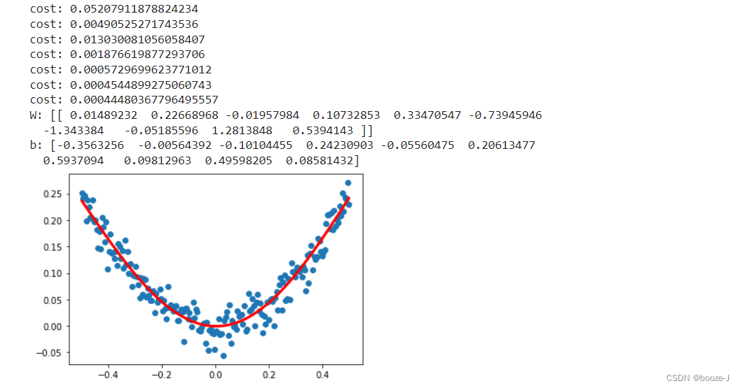
2.非线性回归

Share a latex online editor | with latex common templates

How to write mark down on vscode

How to transfer Netease cloud music /qq music to Apple Music
Su embedded training - Day6
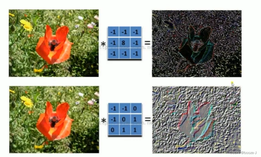
9.卷积神经网络介绍
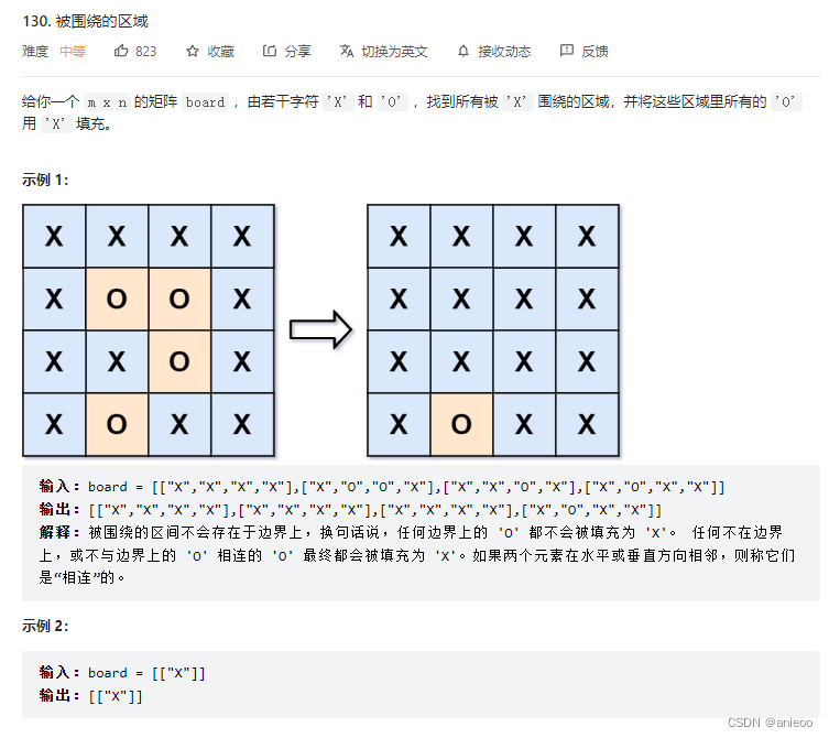
130. Surrounding area
8.优化器
SDNU_ ACM_ ICPC_ 2022_ Summer_ Practice(1~2)
随机推荐
How does starfish OS enable the value of SFO in the fourth phase of SFO destruction?
Service mesh introduction, istio overview
Su embedded training - Day8
letcode43:字符串相乘
第四期SFO销毁,Starfish OS如何对SFO价值赋能?
3. MNIST dataset classification
Redis, do you understand the list
NTT template for Tourism
Codeforces Round #804 (Div. 2)(A~D)
[Yugong series] go teaching course 006 in July 2022 - automatic derivation of types and input and output
新库上线 | CnOpenData中国星级酒店数据
手机上炒股安全么?
Su embedded training - Day6
Using GPU to train network model
Kubernetes static pod (static POD)
Saving and reading of network model
How to use education discounts to open Apple Music members for 5 yuan / month and realize member sharing
完整的模型验证(测试,demo)套路
英雄联盟胜负预测--简易肯德基上校
y59.第三章 Kubernetes从入门到精通 -- 持续集成与部署(三二)