当前位置:网站首页>Data mining - a discussion on sample imbalance in classification problems
Data mining - a discussion on sample imbalance in classification problems
2022-07-06 14:09:00 【DataScienceZone】
When I was looking at some competition cases before, I encountered the imbalance of samples , Tried different sampling methods , It doesn't work very well , So in this article, let's discuss .
1、 Is it necessary to upsample if the sample is unbalanced / Down sampling
1.1 Data preparation
Here we generate a containing 2 Features Of 2 classification Data sets , At the same time, centralize the data 2 The distribution difference of class sample data in the sample space is relatively obvious , The code is as follows :
import pandas as pd
import matplotlib.pyplot as plt
from random import uniform

#  The label is 0 Categories , The first feature is 0~1 Random number between , The second feature is 2~3 Random number between
res1 = []
for i in range(50):
    res1.append([uniform(0,1), uniform(2,3), 0])

#  The label is 1 Categories , The first feature is 2~3 Random number between , The second feature is 0~1 Random number between
res2 = []
for j in range(500):
    res2.append([uniform(2,3), uniform(0,1), 1])

res = res1 + res2

#  hold res convert to Dataframe, And reset the column name
df = pd.DataFrame(res)
df.columns = ['x_1', 'x_2', 'y']

#  Draw a scatter plot of the data set
fig = plt.figure(figsize=(10,6))
plt.scatter(df.x_1, df.x_2)
plt.xlabel('x_1')
plt.ylabel('x_2')
plt.show()
The data generated is as follows (0、1 The proportion of categories is 1:10):
1.2 Training 、 Test the classification effect of the model
Using support vector machine model , Classify the data , And print the evaluation matrix :
from sklearn import svm
from sklearn.model_selection import train_test_split
from sklearn import metrics

#  there df It is generated in the previous step df, Split features and labels
x = df.drop(columns=['y'])
y = df['y']

#  Generating training sets and test sets
x_train, x_test, y_train, y_test = train_test_split(x, y, test_size=0.3, random_state=1)

#  Define and train support vector machine models
clf = svm.SVC()
clf.fit(x_train, y_train)

#  Print the scoring matrix
y_pred = clf.predict(x_test)
print(metrics.classification_report(y_test,y_pred))
The printed scoring matrix is as follows :
              precision    recall  f1-score   support

           0       1.00      1.00      1.00        19
           1       1.00      1.00      1.00       146

    accuracy                           1.00       165
   macro avg       1.00      1.00      1.00       165
weighted avg       1.00      1.00      1.00       165
You can see that the classification effect of the model is very good .
1.3 Draw the classification interval of support vector machine
You can also put the trained model , Draw the classification boundary
import numpy as np


res_new = np.array(res)
x_new = res_new[:,0:2]
y_new = res_new[:,2]

clf = svm.SVC()
clf.fit(x_new, y_new)


fig2 = plt.figure(figsize=(10,6))
plt.scatter(x_new[:, 0], x_new[:, 1], c=y_new, s=30, cmap=plt.cm.Paired)
ax = plt.gca()
xlim = ax.get_xlim()
ylim = ax.get_ylim()

# create grid to evaluate model
xx = np.linspace(xlim[0], xlim[1], 30)
yy = np.linspace(ylim[0], ylim[1], 30)
YY, XX = np.meshgrid(yy, xx)
xy = np.vstack([XX.ravel(), YY.ravel()]).T
Z = clf.decision_function(xy).reshape(XX.shape)

# plot decision boundary and margins
ax.contour(
    XX, YY, Z, colors="k", levels=[-1, 0, 1], alpha=0.5, linestyles=["--", "-", "--"]
)
# plot support vectors
ax.scatter(
    clf.support_vectors_[:, 0],
    clf.support_vectors_[:, 1],
    s=100,
    linewidth=1,
    facecolors="none",
    edgecolors="k",
)
plt.show()
The resulting image is as follows :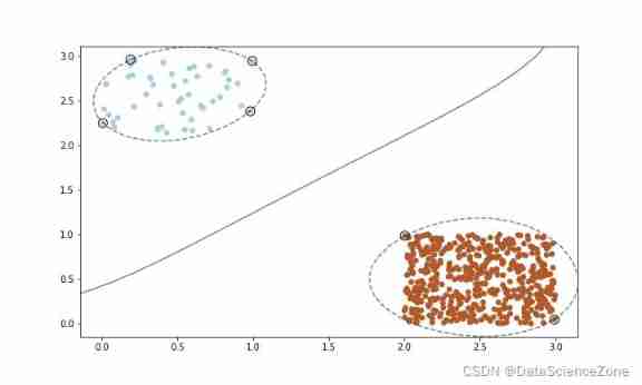
1.4 Conclusion 1
According to the above test , So the conclusion is : If the features in the dataset are well differentiated , The distribution of different types of samples in the sample space can be clearly distinguished , Then even if the sample is unbalanced, it will not affect the classification effect of the model , namely Features determine the upper limit of classification accuracy .
2、 On the sampling / Whether down sampling can really improve the classification effect of the model
2.1 Data preparation
Here is also the generation contains 2 Features Of 2 classification Data sets , The code is as follows :
#  Pour in the required modules
import numpy as np
import matplotlib.pyplot as plt
from sklearn import svm
from sklearn.datasets import make_blobs

# we create two clusters of random points
#  establish 2 Data of class samples , The label is 0 The data of 1000 Bar record , The label is 1 The data of 100 Bar record
n_samples_1 = 1000
n_samples_2 = 100
centers = [[0.0, 0.0], [2.0, 2.0]]
clusters_std = [1.5, 0.5]
X, y = make_blobs(
    n_samples=[n_samples_1, n_samples_2],
    centers=centers,
    cluster_std=clusters_std,
    random_state=0,
    shuffle=False,
)
2.2 Training models
Next, train the support vector machine model , The first model uses sample data directly ; The second model modifies parameters class_weight , To label as 1 Sample up , The code is as follows :
# fit the model and get the separating hyperplane
clf = svm.SVC(kernel="linear", C=1.0)
clf.fit(X, y)

# fit the model and get the separating hyperplane using weighted classes
wclf = svm.SVC(kernel="linear", class_weight={
    1: 10})
wclf.fit(X, y)
2.3 Draw classification boundaries
Then draw 2 Classification boundaries of models , The code is as follows :
# plot the samples
fig3 = plt.figure(figsize=(10,6))
plt.scatter(X[:, 0], X[:, 1], c=y, cmap=plt.cm.Paired, edgecolors="k")

# plot the decision functions for both classifiers
ax = plt.gca()
xlim = ax.get_xlim()
ylim = ax.get_ylim()

# create grid to evaluate model
xx = np.linspace(xlim[0], xlim[1], 30)
yy = np.linspace(ylim[0], ylim[1], 30)
YY, XX = np.meshgrid(yy, xx)
xy = np.vstack([XX.ravel(), YY.ravel()]).T

# get the separating hyperplane
Z = clf.decision_function(xy).reshape(XX.shape)

# plot decision boundary and margins
a = ax.contour(XX, YY, Z, colors="k", levels=[0], alpha=0.5, linestyles=["-"])

# get the separating hyperplane for weighted classes
Z = wclf.decision_function(xy).reshape(XX.shape)

# plot decision boundary and margins for weighted classes
b = ax.contour(XX, YY, Z, colors="r", levels=[0], alpha=0.5, linestyles=["-"])

plt.legend(
    [a.collections[0], b.collections[0]],
    ["non weighted", "weighted"],
    loc="upper right",
)
plt.show()
2.4 Compare the classification effect of the model
Use the model trained in the previous step , Separately predict the labels of the input data ( The data input here is still a training set ), Then print the evaluation matrix , The code is as follows :
from sklearn import metrics

y_pre_1 = clf.predict(X)		#  No upsampling model is used
y_pre_2 = wclf.predict(X)		#  Use the upsampled model

print(metrics.classification_report(y,y_pre_1))
print(metrics.classification_report(y,y_pre_2))
The printed evaluation matrix is as follows :
#  No upsampling model is used
              precision    recall  f1-score   support

           0       0.96      0.98      0.97      1000
           1       0.71      0.59      0.64       100

    accuracy                           0.94      1100
   macro avg       0.84      0.78      0.81      1100
weighted avg       0.94      0.94      0.94      1100

#  Split line ----------------------------------------------
#  No upsampling model is used
              precision    recall  f1-score   support

           0       1.00      0.90      0.95      1000
           1       0.50      0.97      0.66       100

    accuracy                           0.91      1100
   macro avg       0.75      0.94      0.81      1100
weighted avg       0.95      0.91      0.92      1100
You can find 2 Inside the model , The label of the model after sampling is 1 The sample of , The accuracy is down , Recall rate increased .2 A model of f1-score The difference is not obvious , On the whole 2 The effect difference of the two models is not obvious .
2.5 Conclusion 2
Summarize the test results above , We can draw : By up sampling / Down sampling does not necessarily improve the classification effect of the model , However, it can also be sampled when training the model / Down sampling attempt .
3 summary
Data characteristics It is the key to determine the effect of the model .
If there is any mistake in the above discussion , Please also point out that .
Reference link :
https://scikit-learn.org/stable/modules/generated/sklearn.svm.SVC.html#sklearn.svm.SVC
https://scikit-learn.org/stable/auto_examples/svm/plot_separating_hyperplane_unbalanced.html
https://scikit-learn.org/stable/auto_examples/svm/plot_separating_hyperplane.html#sphx-glr-auto-examples-svm-plot-separating-hyperplane-py
边栏推荐
猜你喜欢
Strengthen basic learning records

2. First knowledge of C language (2)
How to turn wechat applet into uniapp
Hackmyvm Target Series (3) - vues
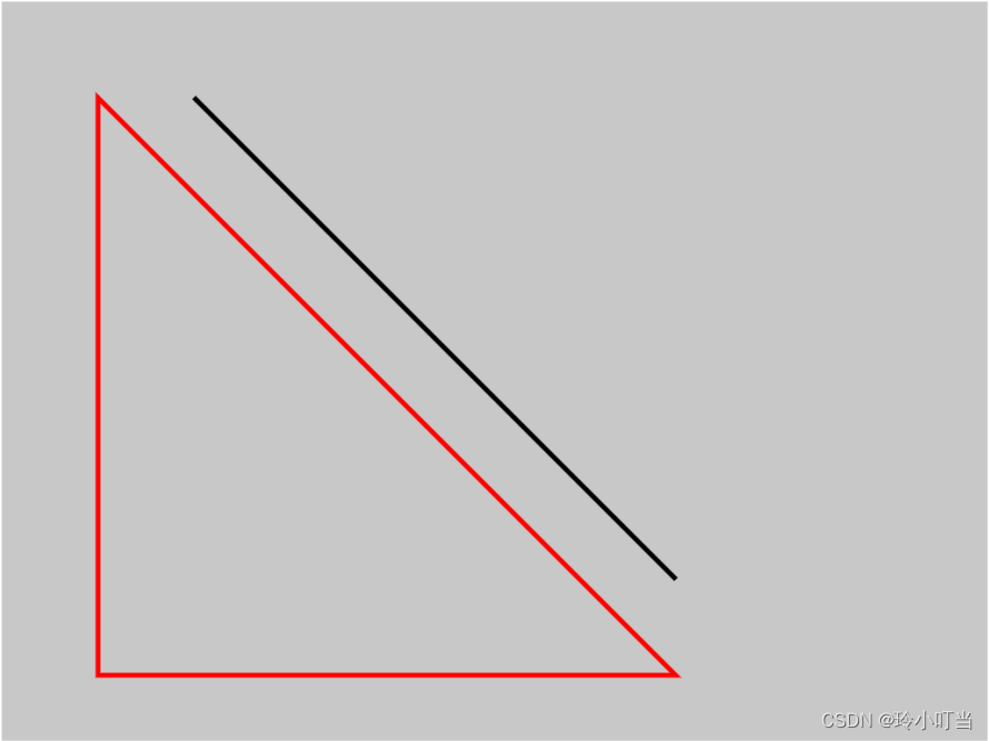
Canvas foundation 1 - draw a straight line (easy to understand)
Ucos-iii learning records (11) - task management
Intranet information collection of Intranet penetration (5)
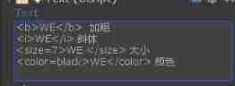
UGUI—Text
Reinforcement learning series (I): basic principles and concepts
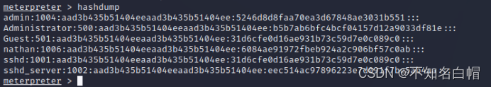
记一次猫舍由外到内的渗透撞库操作提取-flag
随机推荐
Which is more advantageous in short-term or long-term spot gold investment?
Low income from doing we media? 90% of people make mistakes in these three points
4. Branch statements and loop statements
Analysis of penetration test learning and actual combat stage
WEB漏洞-文件操作之文件包含漏洞
实验五 类和对象
7-1 输出2到n之间的全部素数(PTA程序设计)
7-5 走楼梯升级版(PTA程序设计)
The United States has repeatedly revealed that the yield of interest rate hiked treasury bonds continued to rise
《英特尔 oneAPI—打开异构新纪元》
7-7 7003 组合锁(PTA程序设计)
[experiment index of educator database]
1. First knowledge of C language (1)
3. Input and output functions (printf, scanf, getchar and putchar)
实验六 继承和多态
Spot gold prices rose amid volatility, and the rise in U.S. prices is likely to become the key to the future
Relationship between hashcode() and equals()
Wechat applet
Experiment 6 inheritance and polymorphism
Hackmyvm target series (2) -warrior